One of our SQL Server workloads runs many concurrent parallel queries on a possibly already busy server. Other work occurring on the server can have dramatic effects on parallel query runtimes. One way to improve scalability of parallel query runtimes is to achieve query plans with operators that allow a dynamic amount of work to be completed by each parallel worker thread. For example, exchange operators with a partitioning type of hash or round robin force a typically even amount of work to be completed by each worker thread. If a worker thread happens to be on a busy scheduler then query runtime may increase due to the longer runtime of the worker thread that is competing for CPU resources. Serial zones in parallel query plans can of course have the same problem. Batch mode operators, exchange operators with a partitioning type of broadcast or demand, and the parallel page supplier are all examples of operators which can do a dynamic amount of work per thread. Those are the operators that I prefer to see in query plans for this workload.
Very little has been written about exchange operators with a partitioning type of demand, so I forgive you for not hearing of it before today. There is a brief explanation available here, an example of using demand partitioning to improve some query plans involving partitioned tables, and a Stack Exchange answer for someone comparing round robin and demand partitioning. You have the honor of reading perhaps the fourth blog post about the subject.
Start
The demos are somewhat dependent on hardware so you may not see identical results if you are following along. I’m testing on a machine with 8 CPU and with max server memory was set to 6000 MB. Start with a table with a multi-column primary key and insert about 34 million rows into it:
DROP TABLE IF EXISTS #;
CREATE TABLE # (
ID BIGINT NOT NULL,
ID2 BIGINT NOT NULL,
STRING_TO_AGG VARCHAR(MAX),
PRIMARY KEY (ID, ID2)
);

INSERT INTO # WITH (TABLOCK)
SELECT RN, v.v, REPLICATE('REPLICATE', 77)
FROM (
SELECT TOP (4800000) ROW_NUMBER() OVER (ORDER BY (SELECT NULL)) RN
FROM master..spt_values
CROSS JOIN master..spt_values t2
) q
CROSS JOIN (VALUES (1), (2), (3), (4), (5), (6), (7)) v(v);
The query tuning exercise is to insert the ID column and a checksum of the concatenation of all the STRING_TO_AGG values for each ID value ordered by ID2. This may seem like an odd thing to do but it is based upon a production example with an adjustment to not write as much data as the real query. Not all of us have SANs in our basements, or even have a basement. Use the following for the target table:
DROP TABLE IF EXISTS ##;

CREATE TABLE ## (
ID BIGINT NOT NULL,
ALL_STRINGS_CHECKSUM INT
);
Naturally we use SQL Server 2019 CU4 so the STRING_AGG function is available to us. Here is one obvious way to write the query:
INSERT INTO ## WITH (TABLOCK)
SELECT ID, CHECKSUM(STRING_AGG(STRING_TO_AGG , ',') WITHIN GROUP (ORDER BY ID2))
FROM #
GROUP BY ID
OPTION (MAXDOP 8);
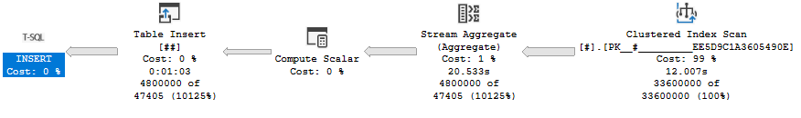
The above query takes about 63 seconds on my machine with a cost of 2320.57 optimizer units. The query optimizer decided that a serial plan was the best choice:
This is a rather lame result for a query tuning exercise so I will assume that I know better and force a parallel query plan with undocumented trace flag 8649. SQL Server warns us that the estimated cost is 4816.68 optimizer units but surely doesn’t expect a detail like that to stop me. The adjusted query executes in 75 seconds:
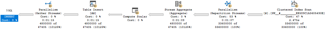
My arrogance is checked. The parallel query is slower than the serial version that the query optimizer wanted us to have. The problem is the hash exchange operator. It is an order preserving exchange with a high MAXDOP and wide rows. This is the worst possible situation for exchange performance. How else can we write the query? Batch mode is not available for STRING_AGG so that’s out. Does anyone remember anything about tuning row mode queries?
The Dark Side
Query hints along with carefully constructed T-SQL are the pathway to many abilities, some considered to be unnatural. We can give the classic Parallel Apply query pattern made famous by Adam Machanic a shot to solve this problem. Perhaps you are thinking that there is no driving table for the outer side of a nested loop join, but we can create one by sampling the clustered index of the base table. I’ll skip that part here and just use what I know about the data to divide it into 96 equal ranges:
DROP TABLE IF EXISTS ###;
CREATE TABLE ### (s BIGINT NOT NULL, e BIGINT NOT NULL);

INSERT INTO ###
VALUES
(1, 50000),
(50001, 100000),
(100001, 150000),
(150001, 200000),
(200001, 250000),
(250001, 300000),
(300001, 350000),
(350001, 400000),
(400001, 450000),
(450001, 500000),
(500001, 550000),
(550001, 600000),
(600001, 650000),
(650001, 700000),
(700001, 750000),
(750001, 800000),
(800001, 850000),
(850001, 900000),
(900001, 950000),
(950001, 1000000),
(1000001, 1050000),
(1050001, 1100000),
(1100001, 1150000),
(1150001, 1200000),
(1200001, 1250000),
(1250001, 1300000),
(1300001, 1350000),
(1350001, 1400000),
(1400001, 1450000),
(1450001, 1500000),
(1500001, 1550000),
(1550001, 1600000),
(1600001, 1650000),
(1650001, 1700000),
(1700001, 1750000),
(1750001, 1800000),
(1800001, 1850000),
(1850001, 1900000),
(1900001, 1950000),
(1950001, 2000000),
(2000001, 2050000),
(2050001, 2100000),
(2100001, 2150000),
(2150001, 2200000),
(2200001, 2250000),
(2250001, 2300000),
(2300001, 2350000),
(2350001, 2400000),
(2400001, 2450000),
(2450001, 2500000),
(2500001, 2550000),
(2550001, 2600000),
(2600001, 2650000),
(2650001, 2700000),
(2700001, 2750000),
(2750001, 2800000),
(2800001, 2850000),
(2850001, 2900000),
(2900001, 2950000),
(2950001, 3000000),
(3000001, 3050000),
(3050001, 3100000),
(3100001, 3150000),
(3150001, 3200000),
(3200001, 3250000),
(3250001, 3300000),
(3300001, 3350000),
(3350001, 3400000),
(3400001, 3450000),
(3450001, 3500000),
(3500001, 3550000),
(3550001, 3600000),
(3600001, 3650000),
(3650001, 3700000),
(3700001, 3750000),
(3750001, 3800000),
(3800001, 3850000),
(3850001, 3900000),
(3900001, 3950000),
(3950001, 4000000),
(4000001, 4050000),
(4050001, 4100000),
(4100001, 4150000),
(4150001, 4200000),
(4200001, 4250000),
(4250001, 4300000),
(4300001, 4350000),
(4350001, 4400000),
(4400001, 4450000),
(4450001, 4500000),
(4500001, 4550000),
(4550001, 4600000),
(4600001, 4650000),
(4650001, 4700000),
(4700001, 4750000),
(4750001, 4800000);
I can now construct a query that gets a parallel apply type of plan:
INSERT INTO ## WITH (TABLOCK)
SELECT ca.*
FROM ### driver
CROSS APPLY (
	SELECT TOP (987654321987654321) ID, CHECKSUM(STRING_AGG(STRING_TO_AGG , ',') WITHIN GROUP (ORDER BY ID2)) ALL_STRINGS_CHECKSUM
	FROM # WITH (FORCESEEK)
	WHERE ID BETWEEN driver.s AND driver.e
	GROUP BY ID
) ca
OPTION (MAXDOP 8, NO_PERFORMANCE_SPOOL, FORCE ORDER);
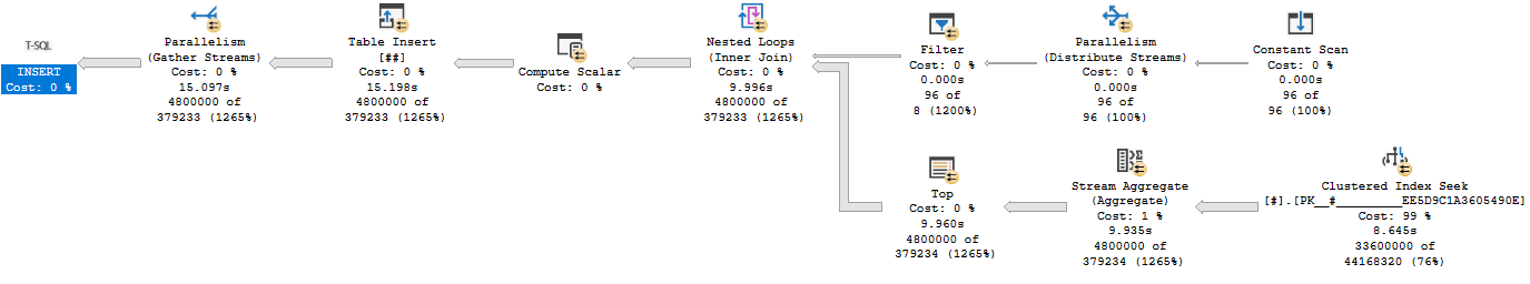
This is an unnatural query plan. The query optimizer assigned it a cost of 36248.7 units. I had to add the TOP to get a valid query plan with an index seek. Removing the TOP operator results in error 8622. Naturally such things won’t stop us and running the query results in an execution time between 15 – 19 seconds on my machine which is the best result yet.
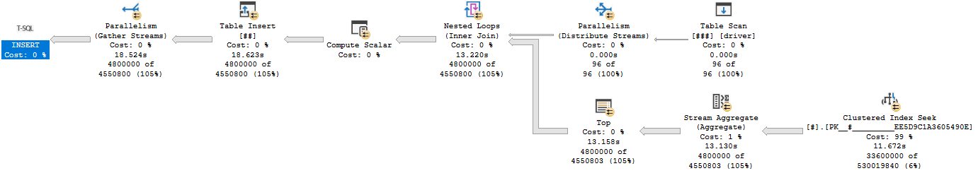
This query plan has an exchange partitioning type of round robin. Recall such exchange types can lead to trouble if there’s other work executing on one of the schedulers used by a parallel worker thread. So far I’ve been testing these MAXDOP 8 queries with nothing else running on my 8 core machine. I can make a scheduler busy by running a MAXDOP 1 query that has no real reason to yield before exhausting its 4 ms quantum. Here is one way to accomplish that:
SELECT TOP (1) t1.high + t2.high + t3.high + t4.high
FROM master..spt_values t1
CROSS JOIN master..spt_values t2
CROSS JOIN master..spt_values t3
CROSS JOIN master..spt_values t4
ORDER BY t1.high + t2.high + t3.high + t4.high
OPTION (MAXDOP 1, NO_PERFORMANCE_SPOOL);
Wait stats for this query if you don’t believe me:
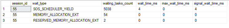
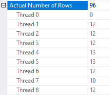
Running this query at the same time as the parallel query can apply a large performance penalty to the parallel query. The parallel query can take up to 48 seconds to execute if even a single worker thread has to share time on a scheduler with another. That is, the query ran 3 times slower when I added a single MAXDOP 1 query to the workload. Looking at thread details for the parallel query:
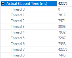
As you can see, one of the worker threads took a significantly longer amount of time to complete its work compared to the other threads. There is no logged wait statistic for this kind of performance problem in which the other parallel worker threads complete their work much earlier than when the query finishes. If there’s no worker thread then there is no wait associated with the query. The only way to catch this is to look at actual row distribution or the CPU time to elapsed time ratio.
You may be wondering why the query is worse than twice as slow as before. After all, if all workers do an equal amount of work but one now gets access to half as much CPU as before it seems reasonable to expect the runtime to double instead of triple. The workers of the parallel query have many reasons they might yield before exhausting their full 4 ms quantum – an I/O wait for example. The MAXDOP 1 SELECT query is designed to not yield early. What is very likely happening is that the MAXDOP 1 query gets a larger share of the scheduler’s resources than 50%. SQL Server 2016 made adjustments to try to limit this type of situation but by its very nature I don’t see how it could ever lead to a perfect sharing of a scheduler’s resources.
Demanding Demand Partitioning
We can get an exchange operator with demand based partitioning by replacing the driving temp table with a derived table. Full query text below:
INSERT INTO ## WITH (TABLOCK)
SELECT ca.*
FROM (
VALUES
(1, 50000),
(50001, 100000),
(100001, 150000),
(150001, 200000),
(200001, 250000),
(250001, 300000),
(300001, 350000),
(350001, 400000),
(400001, 450000),
(450001, 500000),
(500001, 550000),
(550001, 600000),
(600001, 650000),
(650001, 700000),
(700001, 750000),
(750001, 800000),
(800001, 850000),
(850001, 900000),
(900001, 950000),
(950001, 1000000),
(1000001, 1050000),
(1050001, 1100000),
(1100001, 1150000),
(1150001, 1200000),
(1200001, 1250000),
(1250001, 1300000),
(1300001, 1350000),
(1350001, 1400000),
(1400001, 1450000),
(1450001, 1500000),
(1500001, 1550000),
(1550001, 1600000),
(1600001, 1650000),
(1650001, 1700000),
(1700001, 1750000),
(1750001, 1800000),
(1800001, 1850000),
(1850001, 1900000),
(1900001, 1950000),
(1950001, 2000000),
(2000001, 2050000),
(2050001, 2100000),
(2100001, 2150000),
(2150001, 2200000),
(2200001, 2250000),
(2250001, 2300000),
(2300001, 2350000),
(2350001, 2400000),
(2400001, 2450000),
(2450001, 2500000),
(2500001, 2550000),
(2550001, 2600000),
(2600001, 2650000),
(2650001, 2700000),
(2700001, 2750000),
(2750001, 2800000),
(2800001, 2850000),
(2850001, 2900000),
(2900001, 2950000),
(2950001, 3000000),
(3000001, 3050000),
(3050001, 3100000),
(3100001, 3150000),
(3150001, 3200000),
(3200001, 3250000),
(3250001, 3300000),
(3300001, 3350000),
(3350001, 3400000),
(3400001, 3450000),
(3450001, 3500000),
(3500001, 3550000),
(3550001, 3600000),
(3600001, 3650000),
(3650001, 3700000),
(3700001, 3750000),
(3750001, 3800000),
(3800001, 3850000),
(3850001, 3900000),
(3900001, 3950000),
(3950001, 4000000),
(4000001, 4050000),
(4050001, 4100000),
(4100001, 4150000),
(4150001, 4200000),
(4200001, 4250000),
(4250001, 4300000),
(4300001, 4350000),
(4350001, 4400000),
(4400001, 4450000),
(4450001, 4500000),
(4500001, 4550000),
(4550001, 4600000),
(4600001, 4650000),
(4650001, 4700000),
(4700001, 4750000),
(4750001, 4800000)
) driver( s, e)
CROSS APPLY (
	SELECT TOP (987654321987654321) ID, CHECKSUM(STRING_AGG(STRING_TO_AGG , ',') WITHIN GROUP (ORDER BY ID2)) ALL_STRINGS_CHECKSUM
	FROM # WITH (FORCESEEK)
	WHERE ID BETWEEN CAST(driver.s AS BIGINT) AND CAST(driver.e AS BIGINT)
	GROUP BY ID
) ca
OPTION (MAXDOP 8, NO_PERFORMANCE_SPOOL, FORCE ORDER);
Query performance is effectively random. The query was observed to execute as quickly as 15 seconds and as slowly as 45 seconds. In some situations there was an incredible amount of skew in row distributions between threads:

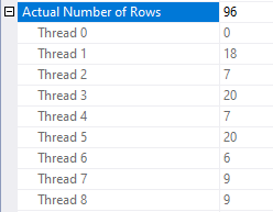

This is an unexpected situation if there are no other queries running on the server. Query performance is most disappointing.
Is there a trace flag?
Yes! The problem here is that the nested loop join uses the prefetch optimization. Paul White writes:
One of the available SQL Server optimizations is nested loops prefetching. The general idea is to issue asynchronous I/O for index pages that will be needed by the inner side — and not just for the current correlated join parameter value, but for future values too.
That sounds like it might be wildly incompatible with a demand exchange operator. Querying sys.dm_exec_query_profiles during query execution proves that the demand exchange isn’t working as expected: worker threads no longer fully process the results associated with their current row before requesting the next one. That is what can lead to wild skew between the worker threads and as a result query performance is effectively random.
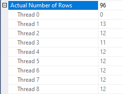
Documented trace flag 8744 disables this optimization. Adding it to the query using QUERYTRACEON results in much more stable performance. The query typically finishes in about 15 seconds. Here is an example thread distribution:
If you fight the ISV fight like I do, you may not be able to enable trace flags for individual queries. If you’re desperate you could try artificially lowering the cardinality estimate from the derived table. An OPTIMIZE FOR query hint with a direct filter is my preferred way to accomplish this. I like to set the cardinality estimate equal to MAXDOP but I have no real basis for doing this. Here is the full query text:
DECLARE @filter BIGINT = 987654321987654321;
INSERT INTO ## WITH (TABLOCK)
SELECT ca.*
FROM (
VALUES
(1, 50000),
(50001, 100000),
(100001, 150000),
(150001, 200000),
(200001, 250000),
(250001, 300000),
(300001, 350000),
(350001, 400000),
(400001, 450000),
(450001, 500000),
(500001, 550000),
(550001, 600000),
(600001, 650000),
(650001, 700000),
(700001, 750000),
(750001, 800000),
(800001, 850000),
(850001, 900000),
(900001, 950000),
(950001, 1000000),
(1000001, 1050000),
(1050001, 1100000),
(1100001, 1150000),
(1150001, 1200000),
(1200001, 1250000),
(1250001, 1300000),
(1300001, 1350000),
(1350001, 1400000),
(1400001, 1450000),
(1450001, 1500000),
(1500001, 1550000),
(1550001, 1600000),
(1600001, 1650000),
(1650001, 1700000),
(1700001, 1750000),
(1750001, 1800000),
(1800001, 1850000),
(1850001, 1900000),
(1900001, 1950000),
(1950001, 2000000),
(2000001, 2050000),
(2050001, 2100000),
(2100001, 2150000),
(2150001, 2200000),
(2200001, 2250000),
(2250001, 2300000),
(2300001, 2350000),
(2350001, 2400000),
(2400001, 2450000),
(2450001, 2500000),
(2500001, 2550000),
(2550001, 2600000),
(2600001, 2650000),
(2650001, 2700000),
(2700001, 2750000),
(2750001, 2800000),
(2800001, 2850000),
(2850001, 2900000),
(2900001, 2950000),
(2950001, 3000000),
(3000001, 3050000),
(3050001, 3100000),
(3100001, 3150000),
(3150001, 3200000),
(3200001, 3250000),
(3250001, 3300000),
(3300001, 3350000),
(3350001, 3400000),
(3400001, 3450000),
(3450001, 3500000),
(3500001, 3550000),
(3550001, 3600000),
(3600001, 3650000),
(3650001, 3700000),
(3700001, 3750000),
(3750001, 3800000),
(3800001, 3850000),
(3850001, 3900000),
(3900001, 3950000),
(3950001, 4000000),
(4000001, 4050000),
(4050001, 4100000),
(4100001, 4150000),
(4150001, 4200000),
(4200001, 4250000),
(4250001, 4300000),
(4300001, 4350000),
(4350001, 4400000),
(4400001, 4450000),
(4450001, 4500000),
(4500001, 4550000),
(4550001, 4600000),
(4600001, 4650000),
(4650001, 4700000),
(4700001, 4750000),
(4750001, 4800000)
) driver( s, e)
CROSS APPLY (
	SELECT TOP (987654321987654321) ID, CHECKSUM(STRING_AGG(STRING_TO_AGG , ',') WITHIN GROUP (ORDER BY ID2)) ALL_STRINGS_CHECKSUM
	FROM # WITH (FORCESEEK)
	WHERE ID BETWEEN CAST(driver.s AS BIGINT) AND CAST(driver.e AS BIGINT)
	GROUP BY ID
) ca
WHERE driver.s <= @filter
OPTION (OPTIMIZE FOR (@filter = 350001), MAXDOP 8, NO_PERFORMANCE_SPOOL, FORCE ORDER);
Query performance is the same as with TF 8744:
Does this query do better than round robin partitioning when there is a busy MAXDOP 1 query running at the same time? I ran it a few times and it completed in about 15-16 seconds every time. One of the worker threads does less work and the others cover for it:
In this example the nested loop join only gets the prefetch optimization if the cardinality estimate is more than 25 rows. I do not know if that number is a fixed part of the algorithm for prefetch eligibility but it certainly feels unwise to rely on this behavior never changing in a future version of SQL Server. Note that prefetching is a trade-off. For some workloads you may be better off with round robin partitioning and prefetching compared to demand without prefetching. It’s hard to imagine a workload that would benefit from demand with prefetching but perhaps I’m not being creative enough in my thinking.
Final Thoughts
In summary, the example parallel apply query that uses demand partitioning performs 2-3 times better the query that uses round robin partitioning when another serial query is running on the server. The nested loop prefetch optimization does not work well witth exchange operator demand partitioning and should be avoided via a trace flag or other tricks if demand partitioning is in use.
There are a few things that Microsoft could do to improve the situation. A USE HINT that disables nested loop prefetching would be most welcome. I think that there’s also a fairly strong argument to make that a query pattern of a nested loop join with prefetching with a first child of a demand exchange operator is a bad pattern that the query optimizer should avoid if possible. Finally, it would be nice if there was a type of wait statistic triggered when some of a parallel query’s workers finish their work earlier than others. The problematic queries here have very little CXPACKET waits and no EXECSYNC waits. Imagine that I put a link to UserVoice requests here and imagine yourself voting for them.
Thanks for reading!
Going Further
If this is the kind of SQL Server stuff you love learning about, you’ll love my training. I’m offering a 75% discount to my blog readers if you click from here. I’m also available for consulting if you just don’t have time for that and need to solve performance problems quickly.
One thought on “Using Exchange Demand Partitioning to Improve Parallel Query Scalability In SQL Server”
Comments are closed.