The NESTING_TRANSACTION_FULL Latch In SQL Server

This blog posts investigates the NESTING_TRANSACTION_FULL latch. This latch class can be a bottleneck in extreme ETL workloads. In case you need a quick definition of a latch:

A latch is a lightweight synchronization object that is used by various SQL Server components. A latch is primarily used to synchronize database pages. Each latch is associated with a single allocation unit. A latch wait occurs when a latch request cannot be granted immediately, because the latch is held by another thread in a conflicting mode. Unlike locks, a latch is released immediately after the operation, even in write operations. Latches are grouped into classes based on components and usage. Zero or more latches of a particular class can exist at any point in time in an instance of SQL Server.

Why is the Latch Needed?


Paul Randal has a good explanation here. My experience with it is isolated to parallel SELECT INTO (introduced in SQL Server 2014) and parallel insert into heaps and columnstore (introduced in SQL Server 2016). Each worker thread of the parallel insert has a subtransaction, but only the main transaction can modify the transaction log. Whenever a worker thread needs to modify the transaction log it needs to take an exclusive latch on a subresource under the NESTING_TRANSACTION_FULL latch class. Only one worker thread can hold the latch for the transaction at a time, so this can lead to contention. This is layperson’s explanation based on observed behavior, so please forgive any inaccuracies.
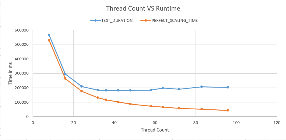
The Test Server


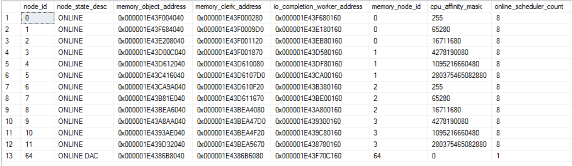
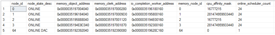
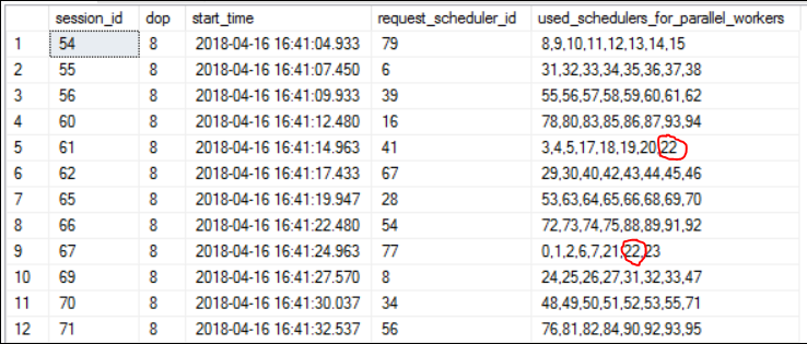
For testing performance and scalability of parallel inserts I prefer to use hardware with a large number of physical cores per socket. I have access to a virtualized test server that’s 4 X 24. I wanted to make tests be as fair as possible, so I decided to only use a single memory node of the server. It seemed logical to pick the node with the least amount of system processes. Here’s a query to view many of them:

SELECT scheduler_id, command
FROM sys.dm_exec_requests r
INNER JOIN sys.dm_exec_sessions s
	ON r.session_id = s.session_id
WHERE s.is_user_process = 0
AND scheduler_id IS NOT NULL
ORDER BY scheduler_id;

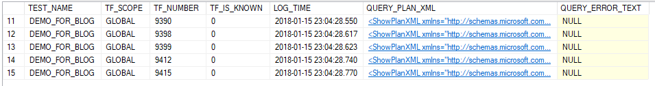
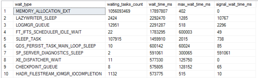
Here is a partial result set:

a32_system_processes

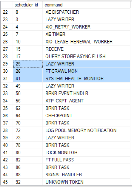
I omitted a few processes such as the LOG WRITERS which are on memory node 0. Memory node 1, which covers schedulers 24 to 47, seems like the best choice. All memory nodes have a LAZY WRITER so that can’t be avoided. I’m not doing any full text work that I’m aware of so that just leaves SYSTEM_HEALTH_MONITOR. We have the best, most healthy systems, so I’m sure that process doesn’t do a lot of work.

Resource governor is always enabled on this server, so I can send new sessions to schedulers on memory node 1 with the following commands:

ALTER RESOURCE POOL [default] WITH
	(AFFINITY SCHEDULER = (24 to 47));

ALTER RESOURCE GOVERNOR RECONFIGURE;

The Table


For testing I wanted to insert a moderate amount of data while varying MAXDOP. I needed to read enough data for parallel table scans to be effective up to MAXDOP 24 and to write enough data so that parallel insert could be effective. At the same time, I didn’t want to write too much data because that could make running dozens of tests impractical.

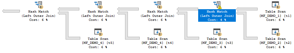
I settled on a two column table with an odd partitioning scheme. All of the data is loaded into a single partition so we can run parallel inserts which result in all rows getting sent to a single thread as needed. Most tests spread rows over all parallel worker threads. The FILLER column is there to give the table enough pages to make parallel scans effective. It’s also helpful to run a slower insert query as needed. Other than that, there’s nothing special about the definition or data of the table and it can be changed as desired.

CREATE PARTITION FUNCTION PF_throwaway_1
(BIGINT)
AS RANGE LEFT
FOR VALUES (0, 1, 2, 3); 

CREATE PARTITION SCHEME PS_throwaway_1
AS PARTITION PF_throwaway_1
ALL TO ( [PRIMARY] );

DROP TABLE IF EXISTS BASE_TABLE;

CREATE TABLE dbo.BASE_TABLE (
	ID BIGINT,
	FILLER VARCHAR(1000)
) ON PS_throwaway_1 (ID);

INSERT INTO dbo.BASE_TABLE WITH (TABLOCK)
SELECT 1, REPLICATE('Z', 100)
FROM master..spt_values t1
CROSS JOIN master..spt_values t2;

The tempdb database seemed like a good target for writes because I already have 96 data files. There also may be some writing optimizations for tempdb which could be helpful.

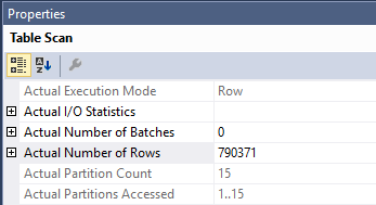
A typical test query for observing latch waits looks like something like this:

SELECT ID, REPLICATE('Z', 1000) COL INTO #t
FROM BASE_TABLE
WHERE ID = 1
OPTION (MAXDOP 1);

With MAXDOP varying all the way from 1 to 24.

How Many Latches are Taken?


sys.dm_os_latch_stats cannot be used to figure out how many total latches were taken:

sys.dm_os_latch_stats does not track latch requests that were granted immediately, or that failed without waiting.

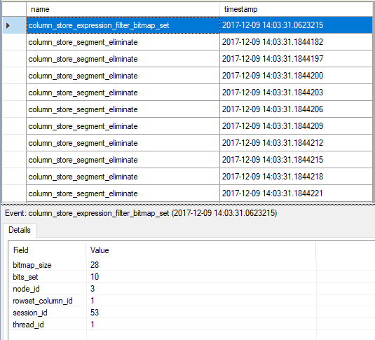
The only way that I know to do that is through extended events. The latch_acquired debug event filtered on the TRAN_NESTING_FULL class is helpful. For data storage targets I used event_counter and histogram. I imagine that these extended events can have a lot of overhead, but I’m doing my testing on a non-production server.

Let’s start with a query that’s not eligible for parallel insert:

DROP TABLE IF EXISTS #t;

SELECT ID, REPLICATE('Z', 1000) COL INTO #t
FROM BASE_TABLE
OPTION (MAXDOP 1);

I expected that no latches will be taken on NESTING_TRANSACTION_FULL. That is indeed what happens.

What about a query that runs at MAXDOP 2 but for which all of the rows are sent to a single worker thread? With four partitions and MAXDOP 2, each worker will be assigned a partition. The worker moves onto the next partition after it reads all of the rows. Skewed data in partitioned tables can lead to parallelism imbalances which can cause problems in real workloads here. It can also be used to our advantage in testing which is what I’m doing here.

DROP TABLE IF EXISTS #t;

SELECT ID, REPLICATE('Z', 1000) COL INTO #t
FROM BASE_TABLE
OPTION (MAXDOP 2);

There is a total of 347435 latch_acquired events for NESTING_TRANSACTION_FULL. The latch was acquired and released 347435 times. If I run a query with rows spread over all parallel workers, such as this one:

DROP TABLE IF EXISTS #t;

SELECT ID, REPLICATE('Z', 1000) COL INTO #t
FROM BASE_TABLE
WHERE ID = 1
OPTION (MAXDOP 2);

I get the same number of latch_acquired events.

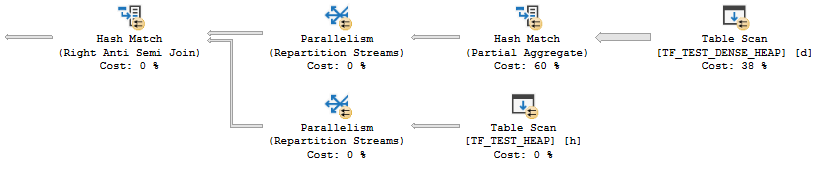
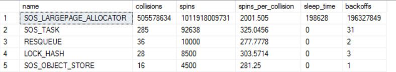
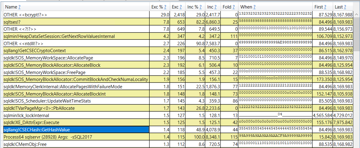
I happened to notice that the query writes 347321 log records to the transaction log. That number is suspiciously close to the number of latches that were acquired. I can get the callstacks around the latch_acquired event by using the technique described here by Jonathan Kehayias. The top three buckets in the histogram each have 115192, 115189, and 115187 events. The callstacks seem to correspond to changing a PFS, GAM, or IAM page. They are reproduced below:

sqlmin.dll!XeSqlPkg::latch_acquired::Publish+0x1a9
sqlmin.dll!LatchBase::RecordAcquire+0x191
sqlmin.dll!LatchBase::AcquireInternal+0x499
sqlmin.dll!ParNestedXdes::GenerateLogRec+0x98
sqlmin.dll!PFSPageRef::ModifyPFSRow+0x68b
sqlmin.dll!ChangeExtStateInPFS+0x2a9
sqlmin.dll!AllocationReq::AllocateExtent+0x33e
sqlmin.dll!AllocationReq::AllocatePages+0x123b
sqlmin.dll!AllocationReq::Allocate+0xf3
sqlmin.dll!ExtentAllocator::PreAllocateExtents+0x457
sqlmin.dll!ExtentAllocatorSingleAlloc::PreAllocate+0x72
sqlmin.dll!ExtentAllocatorSingleAlloc::AllocateExtents+0x26c
sqlmin.dll!CBulkAllocator::AllocateExtent+0x226
sqlmin.dll!CBulkAllocator::AllocatePageId+0xe4
sqlmin.dll!CBulkAllocator::AllocateLinkedAndFormattedLeafPage+0xc1
sqlmin.dll!CHeapBuild::AllocateNextHeapPage+0x1f
sqlmin.dll!CHeapBuild::InsertRow+0x1b1
sqlmin.dll!RowsetBulk::InsertRow+0x23a9
sqlmin.dll!CValRow::SetDataX+0x5b
sqlTsEs.dll!CDefaultCollation::IHashW+0x227
sqlmin.dll!CQScanUpdateNew::GetRow+0x516
sqlmin.dll!CQScanXProducerNew::GetRowHelper+0x386
sqlmin.dll!CQScanXProducerNew::GetRow+0x15
sqlmin.dll!FnProducerOpen+0x5b

sqlmin.dll!XeSqlPkg::latch_acquired::Publish+0x1a9
sqlmin.dll!LatchBase::RecordAcquire+0x191
sqlmin.dll!LatchBase::AcquireInternal+0x499
sqlmin.dll!ParNestedXdes::GenerateLogRec+0x98
sqlmin.dll!PageRef::ModifyBits+0x3e0
sqlmin.dll!ModifyGAMBitAfterNewExtentFound+0xac
sqlmin.dll!AllocExtentFromGAMPage+0x8ef
sqlmin.dll!AllocationReq::AllocateExtent+0x1bb
sqlmin.dll!AllocationReq::AllocatePages+0x123b
sqlmin.dll!AllocationReq::Allocate+0xf3
sqlmin.dll!ExtentAllocator::PreAllocateExtents+0x457
sqlmin.dll!ExtentAllocatorSingleAlloc::PreAllocate+0x72
sqlmin.dll!ExtentAllocatorSingleAlloc::AllocateExtents+0x26c
sqlmin.dll!CBulkAllocator::AllocateExtent+0x226
sqlmin.dll!CBulkAllocator::AllocatePageId+0xe4
sqlmin.dll!CBulkAllocator::AllocateLinkedAndFormattedLeafPage+0xc1
sqlmin.dll!CHeapBuild::AllocateNextHeapPage+0x1f
sqlmin.dll!CHeapBuild::InsertRow+0x1b1
sqlmin.dll!RowsetBulk::InsertRow+0x23a9
sqlmin.dll!CValRow::SetDataX+0x5b
sqlTsEs.dll!CDefaultCollation::IHashW+0x227
sqlmin.dll!CQScanUpdateNew::GetRow+0x516
sqlmin.dll!CQScanXProducerNew::GetRowHelper+0x386
sqlmin.dll!CQScanXProducerNew::GetRow+0x15

sqlmin.dll!XeSqlPkg::latch_acquired::Publish+0x1a9
sqlmin.dll!LatchBase::RecordAcquire+0x191
sqlmin.dll!LatchBase::AcquireInternal+0x499
sqlmin.dll!ParNestedXdes::GenerateLogRec+0x98
sqlmin.dll!PageRef::ModifyBits+0x3e0
sqlmin.dll!ChangeExtStateInIAM+0x2ac
sqlmin.dll!AllocationReq::AllocatePages+0x17e5
sqlmin.dll!AllocationReq::Allocate+0xf3
sqlmin.dll!ExtentAllocator::PreAllocateExtents+0x457
sqlmin.dll!ExtentAllocatorSingleAlloc::PreAllocate+0x72
sqlmin.dll!ExtentAllocatorSingleAlloc::AllocateExtents+0x26c
sqlmin.dll!CBulkAllocator::AllocateExtent+0x226
sqlmin.dll!CBulkAllocator::AllocatePageId+0xe4
sqlmin.dll!CBulkAllocator::AllocateLinkedAndFormattedLeafPage+0xc1
sqlmin.dll!CHeapBuild::AllocateNextHeapPage+0x1f
sqlmin.dll!CHeapBuild::InsertRow+0x1b1
sqlmin.dll!RowsetBulk::InsertRow+0x23a9
sqlmin.dll!CValRow::SetDataX+0x5b
sqlTsEs.dll!CDefaultCollation::IHashW+0x227
sqlmin.dll!CQScanUpdateNew::GetRow+0x516
sqlmin.dll!CQScanXProducerNew::GetRowHelper+0x386
sqlmin.dll!CQScanXProducerNew::GetRow+0x15
sqlmin.dll!FnProducerOpen+0x5b
sqlmin.dll!FnProducerThread+0x80b

The callstack with the next most events only has 472, so I consider those three to be the important ones.

The data for the temp table takes up 7373280 KB of space. That's about 115208 extents, and multiplying that again by 3 is again suspiciously close to the previous two numbers. It seems reasonable to conclude that the number of NESTING_TRANSACTION_FULL latches required for a minimally logged parallel insert into a heap will be approximately equal to 3 times the number of extents needed for the new data. Note that this is an approximation, and there are slight changes to the latch acquire count as MAXDOP changes.

Slowing Down the Insert


I changed the insert query to the following:

DROP TABLE IF EXISTS #t;
SELECT ID
, CASE WHEN CHARINDEX('NO U', FILLER) = 0
THEN REPLICATE('Z', 1000)
ELSE NULL END COL INTO #t
FROM BASE_TABLE
WHERE ID = 1
OPTION (MAXDOP 1);

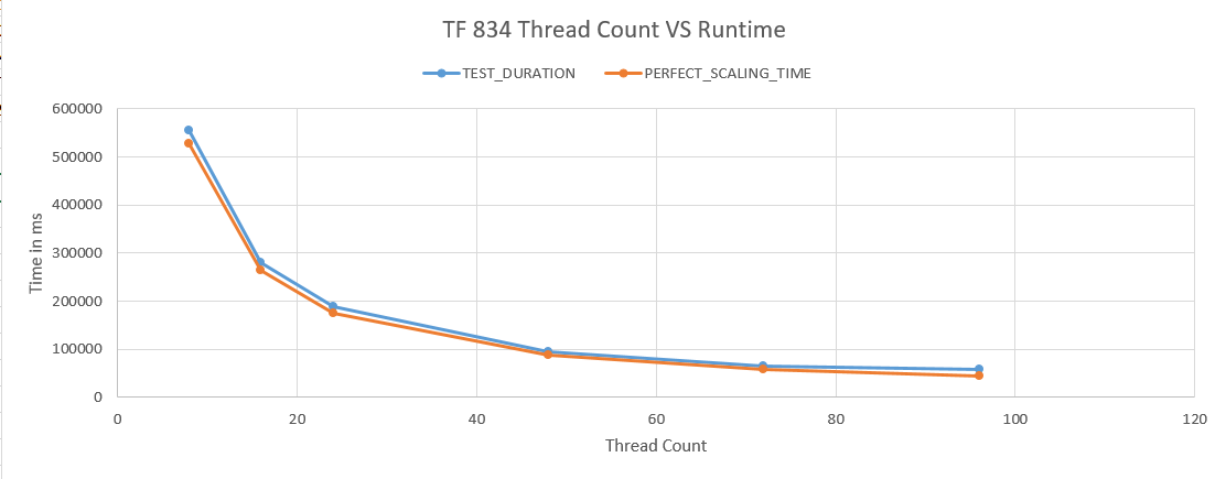
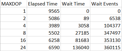
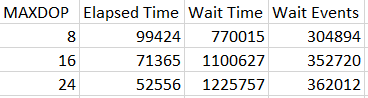
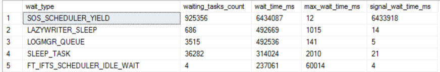
The point is to require more CPU to insert the same volume of data as before. Here is a table showing elapsed time along with wait information for the latch:

a32_slow_no_serial

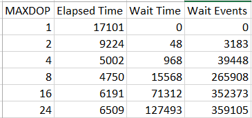
I didn't include CPU time because SET STATISTICS TIME ON was wildly inaccurate for queries with higher DOP. Elapsed time decreases from MAXDOP 1 to MAXDOP 8 but starts to increase after MAXDOP 8. The total wait time dramatically increases as well. In addition, nearly all latch acquires at MAXDOP 16 or MAXDOP 24 had to be waited on.

We know that only one worker can get the exclusive latch for the transaction at a time. Let's use a greatly simplified model for what each parallel worker does for this query. It reads a row, does processing for a row, and goes on to the next one. Once it has enough rows to write out a log record it tries to acquire the latch. If no one else has the latch in exclusive mode it can get the latch, update some structure in the parent transaction, release the latch, and continue reading rows. If another worker has the latch in exclusive mode then it adds itself to the FIFO wait queue for the latch subresource and suspends itself. When the resource is available the worker status changes from SUSPENDED to RUNNABLE. When it changes again from RUNNABLE to RUNNING it acquires the latch, updates some structure in the parent transaction, releases the latch, and continues working until it either needs to suspend again or hits the end of its 4 ms quantum. When it hits the end of its 4 ms quantum it will immediately select itself to run again because there are no other runnable workers on the scheduler.

So what determines the level of contention? One important factor is the number of workers that are contending over the same subresource. For this latch and type of query (rows are pretty evenly distributed between worker threads), this is simply MAXDOP. There's a tipping point for this query where adding more workers is simply counterproductive.

For years I've seen people in the community state that running queries at MAXDOP that's too high can be harmful. I've always been after simple demos that show why that can happen. The NESTING_TRANSACTION_FULL latch is an excellent example of why some queries run longer if MAXDOP is increased too far. There's simply too much contention over a shared resource.

Speeding up the Insert


Let's go back to the original query which is able to insert data at a faster rate:

DROP TABLE IF EXISTS #t;
SELECT ID, REPLICATE('Z', 1000) COL INTO #t
FROM BASE_TABLE
WHERE ID = 1
OPTION (MAXDOP 2);

Here is a table showing elapsed time along with wait information for the latch:

a32_fast_no_serial

We see a similar pattern to the previous query. However, run times are fairly close at MAXDOP 16 and 24. How can that be? Based on the MAXDOP 1 run times we know that this query only has to do about 50% of the CPU work compared to the other query.

Consider the rate of latch acquisition. Let's suppose that we need to take around 360000 latches for both queries and suppose that their parallel workers never need to wait on anything. Based on the MAXDOP 1 runtime for this query we can work at a rate of 360000/(9565/4) = 150 latches per 4 ms quantum per worker. For the slower query, we can only work at a rate of 360000/(17101/4) = 84 latch acquires per 4 ms quantum. Of course, the assumption that none of the workers for these parallel queries will wait is wrong. We can see high wait times at high MAXDOP. The key is to think about what each worker does between waits. It's true that the first query needs to do more CPU work overall. However, at MAXDOP 24 we can have up to 23 workers in the wait queue for the latch. It seems unlikely that a worker will be able to acquire many latches in a row without waiting. At high MAXDOP workers will often need to suspend themselves. As long as the amount of work between log records is significantly less than the 4 ms quantum then there won't be a run time difference between the queries. The query with CHARINDEX will do useful CPU work while the query without it will wait. That's why the query without CHARINDEX has more aggregate wait time at MAXDOP 24. The workers are able to enter a SUSPENDED state faster than the workers for the other queries, but that isn't going to make the query complete any faster.

Adding a Busy Scheduler


In the previous tests we only had a single user query running on the 24 schedulers available to us. That isn't a realistic real world scenario. There will often be other queries competing for CPU resources on the same schedulers. Now I'll add a single MAXDOP 1 query which won't finish its work for many hours. It's designed to burn CPU as efficiently as possible in that there are very few possible waits. The worker thread should be able to use its full 4 ms quantum almost always. Here's the query that I used:

SELECT TOP (1) t1.high + t2.high + t3.high + t4.high
FROM master..spt_values t1
CROSS JOIN master..spt_values t2
CROSS JOIN master..spt_values t3
CROSS JOIN master..spt_values t4
ORDER BY t1.high + t2.high + t3.high + t4.high
OPTION (MAXDOP 1, NO_PERFORMANCE_SPOOL)

I believe the query was assigned to scheduler 27. It stayed there until I cancelled the query.

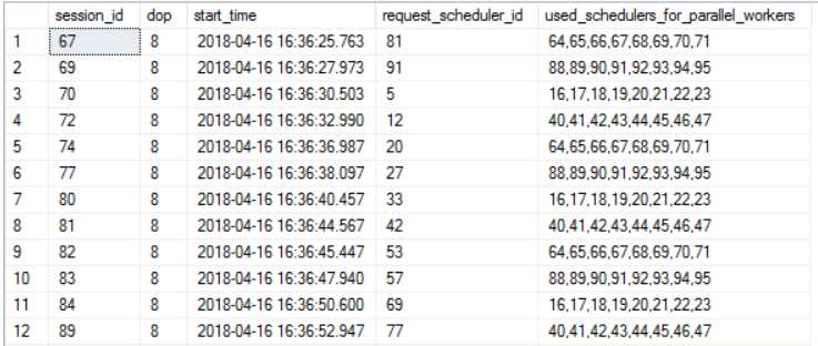
What happens to the performance of the parallel SELECT INTO when one of the schedulers for its workers shares a scheduler with the MAXDOP 1 query? To make that happen I kept track of where the parallel enumerator was and made sure that 8 of the parallel workers were always assigned to the soft-NUMA node which contained the scheduler of the MAXDOP 1 query. I don't love my readers enough to configure soft NUMA so I only have test results for MAXDOP 8, 16, and 24 (auto soft-NUMA splits a virtualized 24 scheduler memory node into 3 groups of 8 schedulers). Here are the test results:

a32_fast_serial

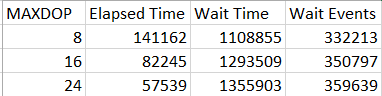
Query run times have dramatically increased. Why did that happen? Recall that latches can be requested at a high rate for the workers of our parallel workers. If a worker requests a latch that it can't get it suspends itself. However, what happens if there's another worker on that same scheduler that can use its full 4 ms quantum, such as our MAXDOP 1 query. Even if the latch resource is available after 1 ms, the worker for the parallel worker won't be able to run for a minimum of 4 ms. It needs to wait for the MAXDOP 1 worker to yield the scheduler. The FIFO nature of the latch queue is harmful here from a query runtime point of view. A scheduling delay between RUNNABLE and RUNNING for a single worker can cause all other parallel worker threads to wait.

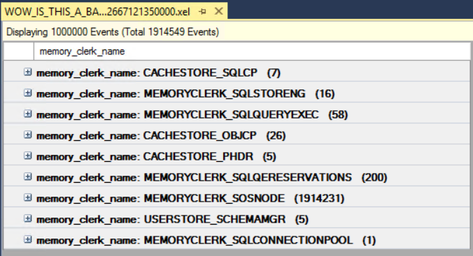
It is interesting that run time gets better with higher MAXDOP. This is the opposite pattern of before. Let's look at the number of latch acquires bucketed by scheduler_id for the MAXDOP 8 query:

a32_fast_interference_schedulers_MAXDOP8

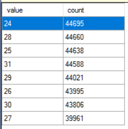
The worker sharing a scheduler with the MAXDOP 1 query does get about 10% fewer latches. However, the FIFO nature of the queue means that work cannot balance well between schedulers, even though the parallel scan and insert operators distribute rows on a demand basis. Based on the wait event counts, it's fair to guess that the worker had to wait on the latch about 33/36 = 91.6% of the time. If the worker on scheduler 27 suspends itself it'll need to wait 4 ms before it can start running again. That gives us a minimum run time for the query of 39961*4*(33/36) = 146523, which is fairly close to the true elapsed time of 141162.

Now consider the latch acquire distribution for the MAXDOP 16 query:

a32_fast_interference_schedulers_MAXDOP16

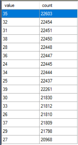
The latches are spread fairly evenly over worker threads. Scheduler 27 only had 20968 latch acquires, so we can calculate our guess for a run time floor as 20968*4*(35/36) = 81542 ms. This is close to the true elapsed time of 82245 ms.

The most important takeaway from this section is that query runtime for parallel inserts or parallel SELECT INTO can dramatically increase if there's any other work happening on those schedulers. Increasing MAXDOP can apparently be helpful in working around scheduler contention, but it will make latch contention worse. I've never seen a practical example where that strategy works out.

Adding More CPU Work


Keeping the busy scheduler, let's go back to the query with CHARINDEX:

DROP TABLE IF EXISTS #t;
SELECT ID
, CASE WHEN CHARINDEX('NO U', FILLER) = 0
THEN REPLICATE('Z', 1000)
ELSE NULL END COL INTO #t
FROM BASE_TABLE
WHERE ID = 1
OPTION (MAXDOP 1);

Here are the test results at MAXDOP 8, 16, and 24:

a32_slow_serial

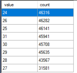
I was surprised to see faster query execution times for the query that effectively needs to do more work. I ran the tests a few times and always saw the same pattern. It certainly makes sense that this query will spend less time on latch waits than the other one, but the exact mechanisms behind faster run times aren't clear to me yet. Here's the count of latches split by worker for the CHARINDEX query:

a32_slow_interference_schedulers_MAXDOP8_compare

Here's the count for a different test run of the query without CHARINDEX:

a32_fast_interference_schedulers_MAXDOP8_compare

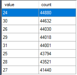
The CHARINDEX query has fewer latch acquires on scheduler 27. That allows the other schedulers to get more latches and to do more work. That explains the difference in run time, but I don't understand why it happens. Perhaps the worker for the CHARINDEX query on scheduler 27 is able to exhaust its 4 ms quantum more often than the other query which allows the other workers to cycle through the latch while the MAXDOP 1 query is on scheduler 27. I may investigate this more another time.

Real World Problems


Adding a single MAXDOP 1 query to the workload in some cases made the parallel query take almost 30 times as long. Is this possible in the real world?

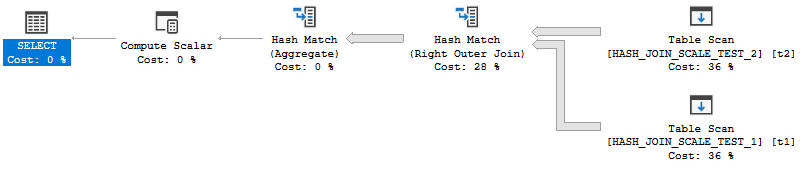
Some parallel inserts generate data to be inserted at a fast rate. Consider the results of a parallel batch mode hash join, for example. Multiple exclusive latches on NESTING_TRANSACTION_FULL seem to be required for every transaction log record that is generated. This can slow down queries and limit overall scalability. The FIFO nature of the queue is especially problematic when there are high signal waits (delays from changing worker status from RUNNABLE to RUNNING). A worker from another query on a scheduler can lead to waits for every parallel worker for an insert or SELECT INTO. There are many reasons for high signal waits: spinlock pressure, some external waits, nonyielding schedulers, and workers that choose not to yield for reasons only known to them. Query performance can degrade even with just a simple query that exhausts its 4 ms quantum every time, as was shown in this blog post.

Lowering MAXDOP can help, but it may not be enough for some workloads. The high rate of exclusive NESTING_TRANSACTION_FULL latch requests feels like a scalability problem that only Microsoft can solve. It would be great if each subtraction was able to update the log and the subtractions could be grouped as needed, such as for query rollback. I can't speak to the complexities in making such a code change.

Final Thoughts


The NESTING_TRANSACTION_FULL latch can be a scalability and performance bottleneck on systems that do many concurrent parallel insert queries or parallel SELECT INTO queries. If you see this bottleneck for your workload, there are a few things that might be helpful to keep in mind:

  1.  The number of latches taken is proportional to the number of log records needed for the transaction. With minimal logging, the number of exclusive latches taken is about equal to 3 * number of extents.
  2. Latch contention gets worse as MAXDOP increases.
  3. Latch contention gets worse as the rate of latch requests increases. In other words, queries that can generate their data to be inserted very efficiently are more impacted.
  4. Delays keeping parallel workers from moving to RUNNING from the RUNNABLE queue for even one parallel worker can have a disastrous effect on query performance. There are many possible scenarios in which this can happen.

Thanks for reading!

Going Further


If this is the kind of SQL Server stuff you love learning about, you'll love my training. I'm offering a 75% discount to my blog readers if you click from here. I'm also available for consulting if you just don't have time for that and need to solve performance problems quickly.

HASHBYTES Scalability In SQL Server 2017

This blog post explores the scalability of the HASHBYTES function in SQL Server 2017 CU7.

Test Query


Start by putting 11 million rows into a heap. I don’t think that the value for the ID column particularly matters.

DROP TABLE IF EXISTS HB_DEMO;

CREATE TABLE HB_DEMO (ID VARCHAR(10));

INSERT INTO HB_DEMO WITH (TABLOCK)
SELECT TOP (11000000) '0'
FROM master..spt_values t1
CROSS JOIN master..spt_values t2
CROSS JOIN master..spt_values t3
OPTION (MAXDOP 1);

The test query that I’ll be running is the following:

SELECT MAX(HASHBYTES('SHA2_256', R1.ID))
FROM HB_DEMO R1
OPTION (MAXDOP 1);

The purpose of the MAX aggregate is to limit the size of the result set. This is a cheap aggregate because it can be implemented as a stream aggregate. The operator can simply keep the maximum value that it’s found so far, compare the next value to the max, and update the maximum value when necessary. On my test server, the query takes about 20 seconds. If I run the query without the HASHBYTES call it takes about 3 seconds. That matches intuitively what I would expect. Reading 11 million rows from a small table out of the buffer pool should be less expensive than calculating 11 million hashes.

From my naive point of view, I would expect this query to scale well as the number of concurrent queries increases. It doesn’t seem like there should be contention over any shared resources, so as long as every query gets on its own scheduler I wouldn’t expect a large degradation in overall run time as the number of queries increases.

A Trillion Spins


Putting that theory to the test, I kicked off 96 concurrent queries using SQLCMD. The server has 96 CPUs and I verified that each session went to its own scheduler. The overall run time was about 8 minutes instead of the expected 20 seconds. That’s a 24X performance degradation at scale. Both resource monitor and SQL Server claim that CPU is used at a very high rate. There are effectively no latch waits. The only notable wait is 4684777 ms of MEMORY_ALLOCATION_EXT, which seems like a lot, but it only works out to 10% of the workload time because I’m running 96 concurrent queries. As is, I can only account for 15% of the workload time through waits and expected CPU utilization of the queries. However, spinlocks have quite a story to tell:

a31_spins

That’s a trillion spins on SOS_LARGEPAGE_ALLOCATOR in about eight minutes. It’s very hard to say that a specific number of spins, backoffs, or anything else related to spinlocks is “bad”. I view this as a sign of a potential problem because I can’t account for the workload time in any other way, the number of spins is so far ahead of second place, and I’ve run a lot of extreme workloads on this server and have never seen spins or backoffs approach levels like this in such a short period of time.

You may be wondering due to the LARGEPAGE part of the name if I have trace flag 834 enabled. I do not. SQL Server can use large pages for some internal structures even without TF 834. It just can’t use them for the buffer pool. This only works when LPIM is enabled, so a natural troubleshooting step is to disable LPIM.

A More Conventional Approach


With the conventional memory mode, the SOS_LARGEPAGE_ALLOCATOR spinlock disappears. This might seem like a good thing, but the workload still has the same scalability problems as before. The overall run still takes about eight minutes. MEMORY_ALLOCATION_EXT is by far the most prevalent wait:

a31_waits_96

However, wait times only account for about a third of overall workload time. This does seem like an important clue, but I’m unable to source the full workload time to anything visible within SQL Server.

Sometimes SQL Server Doesn’t Tell the Whole Truth


This feels like a good use case for ETW tracing in windows. Resource monitor suggests that SQL Server is using a lot of CPU time, but I don’t know how to account for that CPU time within SQL Server. PerfView can be used to analyze call stacks and to see how much CPU time is spent on different parts of the code. This blog post isn’t a tutorial on how to use PerfView with SQL Server. I’m very inexperienced with the program and can barely manage to get results. This might be because I refused to watch the tutorial video.

I wanted the first test to be a baseline. I gathered data over a handful of seconds while running just a single query in SQL Server. To be clear, this testing was done with the conventional memory manager. Here is a screenshot of the CPU stacks:

a31_perfview_1

If I’m interpreting the data correctly, 29% of CPU time was spent on bcrypt (I assume this is a windows assembly that HASHBYTES calls) and 49% of the time was spent in some way getting the hash value. That’s lower than I expected based on earlier testing results, but I am tracing a 96 core server and some of those other 95 cores will be doing things even if I’m not running user queries on them.

The second test was with 96 concurrent queries. I again gathered data over a handful of seconds, but didn’t take care to sample the exact same number of seconds. Here is a screenshot of the CPU stacks for the 96 query test:

a31_perfview_96

95% of the work done the server involves the HASHBYTES calls. That makes sense, but within those calls there’s a large amount of time spent allocating and deallocating pages. That wasn’t expected, especially because none of my queries even ask for a memory grant. However, I can finally account for the unexpected CPU time. Perhaps the MEMORY_ALLOCATION_EXT wait event is more important than I realized. It may be useful to try to look at page allocations within SQL Server.

Unreasonable Extended Events


The only way I know to track page allocations is through extended events. There’s an extended event called page_allocated with the following description: “Occurs when memory page is allocated”. I can’t imagine ever enabling this on a production server, but I’m on a development server and I don’t care about overhead. I created the event session with a scary sounding name, turned it on, ran a single query on an 11 million row table, and turned it off. That alone generated over 1.2 GB of data. The total number of events logged was 11003143, which almost perfectly matches with one allocation per row in the table. I can group by memory clerk to figure out what is doing the allocations:

a31_XE

I’m able to find that clerk in one of the memory DMVs:

SELECT *
FROM sys.dm_os_memory_clerks c
where c.type = 'MEMORYCLERK_SOSNODE';

However, I’m unable to figure out how to do anything useful with those DMVs. It seems odd to me that memory clerks have one row per soft NUMA node instead of per hard NUMA node, but I can’t say anything more on that subject.

Putting everything together that we’ve seen so far, each call to the HASHBYTES function requires a call to something in the Windows assembly bcrypt. To execute the code in Windows, the MEMORYCLERK_SOSNODE memory clerk within SQL Server needs to allocate and deallocate a page. Allocating and deallocating one page per row may not be a problem when running just one query, but it can lead to contention when running lots of queries. That contention may present itself within SQL Server as the MEMORY_ALLOCATION_EXT external wait type. On servers with LPIM enabled, this could be a large page and can result in trillions of spins on the SOS_LARGEPAGE_ALLOCATOR spinlock.

It may not be a coincidence that in total the workload does over a billion hashes and the total number of wait events for MEMORY_ALLOCATION_EXT is close to that.

What About Call Stacks?


We can get call stacks through Extended Events to further validate the theory. There are two possible triggers: page allocation and an external wait on MEMORY_ALLOCATION_EXT. For both triggers I see the same pattern in the call stack:

sqldk.dll!MemoryClerkInternal::AllocatePagesWithFailureMode+0x2ec
sqldk.dll!MemoryClerkInternal::AllocatePages+0x28
sqldk.dll!TVarPageMgr<0>::PviNewVarPage+0x36
sqldk.dll!TVarPageMgr<0>::PbAllocate+0x1e2
sqldk.dll!CMemObj::Alloc+0x47
sqllang.dll!CSECHash::GetHashValue+0x307
sqllang.dll!GetHashValue+0x25
sqllang.dll!HashBytes+0xb4
sqllang.dll!BytHashBytesByt+0xe3

I interpret that to mean that SQL Server needs to allocate a page for each execution of the HASHBYTES function. It isn’t conclusive evidence but it does match everything else that’s been observed so far.

Final Thoughts


I’m not able to find a workaround for this scalability problem. It’s unfortunate that SQL Server reports full CPU utilization when it experiences this contention. Without LPIM and a complete understanding of expected run time for queries running on the system, an administrator may underestimate the importance of the MEMORY_ALLOCATION_EXT wait times. I was able to observe contention even when running just a few queries at a time, both on the test server and on my laptop. It is even more difficult to observe the problem within SQL Server when running just a few queries. I don’t understand everything that’s involved, but it’s hard not to conclude that HASHBYTES could see significantly improved scalability if it wasn’t necessary to allocate and deallocate a page for every execution of the function.

Thanks for reading!

Going Further


If this is the kind of SQL Server stuff you love learning about, you’ll love my training. I’m offering a 75% discount to my blog readers if you click from here. I’m also available for consulting if you just don’t have time for that and need to solve performance problems quickly.

Automatic Soft-NUMA and SOS_SCHEDULER_YIELD Waits In SQL Server

Auto soft-NUMA can lead to increased SOS_SCHEDULER_YIELD waits on large systems with limited concurrency of large parallel queries. This blog post contains a reproduction of the issue and a brief analysis. I hope any readers from Microsoft appreciate my restraint in not making an “It Just Runs Slower” joke.

What is Auto Soft-NUMA?


Auto soft-NUMA was released in SQL Server 2016 and it is automatically turned on. However, it only has an effect if SQL Server is able to detect that a socket has 9 or more cores. The documentation isn’t very precise in some places and is outright misleading in others, but the Microsoft docs page is a good starting point for readers not familiar with it. For a very quick summary, schedulers in a memory node are split into soft-NUMA groups depending on the total number of schedulers and whether or not SQL Server can detect hyperthreading.

Microsoft expects auto soft-NUMA to improve scalability and performance for most workloads. They don’t really explain this idea in detail, but they do talk about how certain internal structures are partitioned by soft-NUMA node and that partitioning can be helpful for large systems.

This might not be what they mean, but there is one LOG WRITER system process per soft-NUMA node on SQL Server 2016 up to a maximum of 4. All of the log writers aren’t spread over multiple NUMA nodes though. To give an example, a single socket 32 core server will have one log writer process without auto soft-NUMA. With auto soft-NUMA there will be four soft-NUMA nodes, and as a consequence, four log writer processes on CPUs 1-4. That might be beneficial for some workloads.

Another observable behavior change caused by soft-NUMA nodes is differences in scheduling. The effect on scheduler assignment for MAXDOP 1 queries is well-known, but there are more subtle issues that can arise when running parallel queries.

The Test Server


The test server was a VM with 96 cores on four physical NUMA nodes. The VM was the only guest on the physical host and the virtual layout matched the physical layout. Within SQL Server, there are 96 schedulers and 4 memory nodes. Each memory node is split into 3 soft-NUMA nodes of 8 schedulers because SQL Server can’t tell if hyperthreading is enabled and 8 divides evenly into 24. Here’s the output of sys.dm_os_nodes with auto soft-NUMA enabled:

a30_auto_soft_numa_dmv

Server MAXDOP is set to 8. In theory, this should be the ideal setup. Microsoft says that they find eight to be the magic number when it comes to scalabilty of parallel processes. If auto soft-NUMA is disabled then there are only four NUMA nodes with one for each memory node. Here’s the output of sys.dm_os_nodes with auto soft-NUMA disabled:

a30_no_auto_soft_numa_dmv

The Test Code


For the test code, I wanted an easy way to alternate sets of parallel queries that finish very quickly with parallel queries that take a long time to finish. I ended up creating a simple stored procedure that only uses the spt_values table and kicks off a user-specified number of parallel queries that finish nearly instanteously followed by a query that cross joins millions of rows together. The final query in the procedure won’t finish in a reasonable amount of time. it is designed to be cancelled. The idea here is to give the observer as much time as needed to poke around various DMVs to make notes about how threads were scheduled.

CREATE OR ALTER PROCEDURE
[dbo].[RUN_SET_OF_QUERIES] (@num_cheap_queries INT) AS
BEGIN
	SET NOCOUNT ON;

	DECLARE @dummy INT,
	@queries_run_so_far INT = 0,
	@filter INT = 0;

	WHILE @queries_run_so_far
		BETWEEN 0 AND @num_cheap_queries - 1
	BEGIN
		SELECT @dummy = MAX(t1.high + t2.high)
		FROM master..spt_values t1
		CROSS JOIN master..spt_values t2
		WHERE @filter = 1
		OPTION (MAXDOP 8);

		SET @queries_run_so_far = @queries_run_so_far + 1;
	END;

	SELECT @dummy =
	MAX(t1.high + t2.high + t3.high + t4.high)
	FROM master..spt_values t1
	CROSS JOIN master..spt_values t2
	CROSS JOIN master..spt_values t3
	CROSS JOIN master..spt_values t4
	OPTION (MAXDOP 8);
END;

To that end, I chose to execute the stored procedure through sqlcmd. The expensive queries don’t modify data so it’s very fast to cancel all of the in-progress queries by closing the sqlcmd window. Readers following along with their 96 core servers at home should feel free to use whatever methodology they wish to kick off the stored procedures. I found it important to be able to kick off the stored procedure with a user-defined time delay between executions and to not have to wait on the completion of the stored procedure before sending more queries. Below is example syntax for a batch file which kicks off four stored procedure calls with a delay of about 2.5 seconds between each call. Each stored procedure executes two fast parallel queries before executing the very expensive one.

START /B sqlcmd -d {{db_name}} -S {{server_name}} -Q "EXEC [dbo].[RUN_SET_OF_QUERIES] @num_cheap_queries=2" > nul
ping 192.2.0.1 -n 1 -w 2500 > nul
START /B sqlcmd -d {{db_name}} -S {{server_name}} -Q "EXEC [dbo].[RUN_SET_OF_QUERIES] @num_cheap_queries=2" > nul
ping 192.2.0.1 -n 1 -w 2500 > nul
START /B sqlcmd -d {{db_name}} -S {{server_name}} -Q "EXEC [dbo].[RUN_SET_OF_QUERIES] @num_cheap_queries=2" > nul
ping 192.2.0.1 -n 1 -w 2500 > nul
START /B sqlcmd -d {{db_name}} -S {{server_name}} -Q "EXEC [dbo].[RUN_SET_OF_QUERIES] @num_cheap_queries=2" > nul
ping 192.2.0.1 -n 1 -w 2500 > nul


Finally, I needed a query to examine the distribution of parallel workers on the system. In general, you want your parallel workers to be spread out enough so that all schedulers are able to do some useful work. I used the following to get an idea of parallel worker distribution:

SELECT
  session_id
, dop
, start_time
, request_scheduler_id
, STRING_AGG
	(
	CASE WHEN exec_context_id = 0
	THEN NULL ELSE scheduler_id END
	, ','
	)
	WITHIN GROUP (ORDER BY scheduler_id)
	AS used_schedulers_for_parallel_workers
FROM
(
	SELECT
	  dot.session_id
	, dot.scheduler_id
	, dot.exec_context_id
	, req.scheduler_id AS request_scheduler_id
	, req.command
	, req.dop
	, req.start_time
	, dos.parent_node_id
	, dos.cpu_id
	, dos.is_idle
	, dos.load_factor
	, dos.active_workers_count
	FROM
	(
		SELECT DISTINCT
		  session_id
		, scheduler_id
		, exec_context_id
		FROM sys.dm_os_tasks
	) dot
	LEFT OUTER JOIN sys.dm_exec_requests req
		ON dot.session_id = req.session_id
			AND req.request_id = 0
	LEFT OUTER JOIN sys.dm_exec_sessions ses
		ON dot.session_id = ses.session_id
	LEFT OUTER JOIN sys.dm_os_schedulers dos
		ON dos.scheduler_id = dot.scheduler_id
	WHERE ses.is_user_process = 1
) t
GROUP BY
  session_id
, dop
, start_time
, request_scheduler_id
ORDER BY start_time
OPTION (MAXDOP 1);

This query is lazy in that it doesn’t handle plans with multiple parallel zones correctly. However, it works well enough for tests on simple parallel queries (such as the ones for the reproduction forthis post) or for properly written batch mode queries.

Testing with Auto Soft-NUMA


As a reminder, with auto soft-NUMA on my server I had 12 soft-NUMA nodes of 8 schedulers. I restarted SQL Server and ran a .bat file with the following commands repeated 12 times:

START /B sqlcmd -d {{db_name}} -S {{server_name}} -Q "EXEC [dbo].[RUN_SET_OF_QUERIES] @num_cheap_queries=2" > nul
ping 192.2.0.1 -n 1 -w 2500 > nul

In other words, I kicked off a total of 24 very fast parallel queries and 12 very long running parallel queries. Here is how my scheduling of parallel workers looked:

a30_auto_soft_numa_scheduling

That is a pretty bad outcome. I have 12 MAXDOP 8 queries with all parallel workers assigned to schedulers on just four NUMA nodes. Each CPU in those NUMA nodes has the equivalent of 300% work assigned to it. Execution context 0 doesn’t do much work for the test query, so I have 64 cpus with barely any work to do. It’s unlikely that server CPU will go much higher than 33%. Here are wait stats after running the workload for two minutes:

a30_more_sos_waits

We accumulated two hours of SOS_SCHEDULER_YIELD waits in just two minutes. Not what you want to see with a server that’s around 33% CPU utilization. What went wrong?

Mo’ Schedulers Mo’ Problems


Scheduling of parallel queries was changed in SQL Server 2012. Bob Dorr blogged about it here, and it’s the best source that I’m aware of. Even so, I’ve had a lot of trouble figuring out exactly what the words in that blog post mean. Readers of this blog may be able to relate. I’ve only ever observed the spread selection type in practice, so the most relevant part of the linked post is this one:

Spread: This is the most common decision made by SQL Server. The decision spreads the workers across multiple nodes as required. The design is similar to full except the starting position is based on the saved, next node, global enumerator.

Consider a server with soft-NUMA nodes of 8 schedulers with MAXDOP 8. The first parallel query will be sent to numa node 0. The number of active workers matches the number of schedulers exactly so each active worker is assigned to a different scheduler in the NUMA node. The second parallel query will be sent to NUMA node 1. The third parallel query will be sent to NUMA node 2, and so on. Execution of serial queries or creation of sessions does not matter. That advances a counter that’s separate from the “global enumerator” used for parallel query scheduler placement. As far as I can tell the scheduler assigned to execution context 0 does not affect the scheduling of the parallel worker threads, although it can certainly affect parallel query performance.

The scenario described above doesn’t sound so bad. It can work well if the parallel queries take roughly about the same amount of time to complete and query MAXDOP matches the number of schedulers per soft-NUMA node. Problems can emerge when at least one of those is not true. With the spread selection type it’s possible that the amount of work already assigned to schedulers has no effect on parallel query scheduler placement. Let that sink in. You could have 100 serial queries all assigned to schedulers in numa node 0 but SQL Server may still send a parallel query to that NUMA node. It depends on the position of the “global enumerator” as opposed to current work on the server.

That behavior is why the reproduction in this post works. With a total of 12 soft-NUMA nodes all I need to do is run queries in a fast-fast-slow pattern to cause the slow queries to be doubled and tripled up on schedulers. In some cases sending more parallel queries to a server can be a valid strategy if server CPU isn’t quite as high as you’d like. That might not work here though. Sending more queries will mostly just rack up additional SOS_SCHEDULER_YIELD waits.

It isn’t true that SQL Server never considers the amount of work on a scheduler when assigning parallel worker threads. NUMA nodes have limits on the number of parallel workers as can be seen in sys.dm_exec_query_parallel_workers. There appears to be scheduling choices which consider load factor or worker count when the set of parallel workers only fills part of a soft-NUMA node. Consider a pair of MAXDOP 12 queries running on the same server as described earlier. Suppose that the “global enumerator” starts at position 0. The first query will grab 8 schedulers from NUMA node 0 and 4 schedulers from NUMA node 1. SQL Server has some choice about which schedulers it grabs from NUMA node 1. However, there is no choice to be made for NUMA node 0 because it grabs all of them. The second parallel query grabs 4 schedulers from NUMA node 1 and 8 schedulers from NUMA node 2. Again, SQL server can make a choice about which schedulers it uses from NUMA node 1. That decision can factor in system load. Just like with serial queries, if queries are sent too quickly to the server then you might see unnecessary doubling up of schedulers in NUMA node 1.

I didn’t try to dig into the details fully, but hopefully the above gives you a high level understanding of what kind of problems you might see with parallel query scheduling on servers with more than one NUMA node.

Testing Without Auto Soft-NUMA


Armed with our new knowledge, let’s consider what might happen with the previous workload if auto soft-NUMA is disabled. Assume that the server was restarted and the global enumerator starts at position 0. Three MAXDOP 8 queries are able to fit into each NUMA node of 24 schedulers. The expensive query for the first execution of the stored procedure will be sent to schedulers on the first NUMA node. The expensive query for the second execution of the stored procedure will be sent to schedulers on the second NUMA node, the third will be sent to the third NUMA node, and the fourth will be sent to the fourth NUMA node. As we continue to execute more queries we’ll loop around but the key difference is that SQL Server is able to place the parallel worker threads however it wants on the 24 schedulers. It can look at things like load factor or the number of workers per scheduler. After all 12 stored procedures have started we can end up with scheduling like this:

a30_good_scheduling

Every scheduler has at least one thread for a parallel worker or an execution context 0 thread. Scheduler 22 is one of eight schedulers with more than one parallel worker assigned. Execution context 0 for these queries is expected to do very little work, so it could be argued that a better distribution would be to have exactly one parallel worker per scheduler. However, overall this is a pretty good distribution and we can push server CPU to 90%. After two minutes of execution we have significantly fewer time spent on SOS_SCHEDULER_YIELD waits compared to before:

a30_less_sos_waits

In this situation, we can see a significant improvement in server resource utilization by disabling auto soft-NUMA. For other workloads and query mixes the scheduling behavior offered with auto soft-NUMA may be a better fit. Key factors include the patttern of parallel queries, MAXDOP, and the number of schedulers per memory node.

Final Thoughts


We observed a bottleneck with SOS_SCHEDULER_YIELD waits for an ETL workload for which it was not easy to scale up the number of queries. This can happen if there are only so many partitions to process or if ETL queries require large memory grants, say, for compressing columnstore data. We were able to shave 30% off the overall workload time by using Resource Governor CPU affinity and doing our own scheduling. Less drastic workarounds include disabling auto soft-NUMA, changing MAXDOP, increasing CTFP, or reigning in some queries which don’t need to run in parallel. Thanks for reading!

A Row Goal Riddle In SQL Server

I’m the kind of guy who sometimes likes to look at execution plans with different hints applied to see how the plan shape and query operator costs change. Sometimes paying attention to operator costs can provide valuable clues as to why the query optimizer selected a plan that you didn’t like. Sometimes it doesn’t. My least favorite scenario is when I see inconsistent operator costs. This blog post covers a reproduction of such a case involving the dreaded and feared row goal.

The Data


For the data in my demo tables, I wanted a query of the following form:

SELECT *FROM dbo.OUTER_HEAP oWHERE NOT EXISTS(SELECT 1FROM dbo.INNER_CI iWHERE i.ID = o.ID);

that returned zero rows. However, I wanted the query optimizer to think that a decent number of rows would be returned. This was more difficult to do than expected. I could have just hacked stats to easily accomplish what I wanted, but did not do so out of stubbornness and pride. I eventually found a data set through trial and error with a final cardinality estimate of 16935.2 rows, or 1.7% of the rows in the outer table:

DROP TABLE IF EXISTS dbo.OUTER_HEAP;CREATE TABLE dbo.OUTER_HEAP (ID VARCHAR(10));INSERT INTO dbo.OUTER_HEAP WITH (TABLOCK)SELECT TOP (1000000) 1500000+ ROW_NUMBER() OVER (ORDER BY (SELECT NULL))FROM master..spt_values t1CROSS JOIN master..spt_values t2OPTION (MAXDOP 1);CREATE STATISTICS S1 ON dbo.OUTER_HEAP (ID)WITH FULLSCAN;DROP TABLE IF EXISTS dbo.INNER_CI;CREATE TABLE dbo.INNER_CI (ID VARCHAR(10),PRIMARY KEY (ID));INSERT INTO dbo.INNER_CI WITH (TABLOCK)SELECT TOP (2000000) 500000+ ROW_NUMBER() OVER (ORDER BY (SELECT NULL))FROM master..spt_values t1CROSS JOIN master..spt_values t2OPTION (MAXDOP 1);CREATE STATISTICS S1 ON dbo.INNER_CI (ID)WITH FULLSCAN;

The actual query of interest is the following one:

SELECT TOP (1) 1FROM dbo.OUTER_HEAP oWHERE NOT EXISTS(SELECT 1FROM dbo.INNER_CI iWHERE i.ID = o.ID);

Such a query might be used as part of an ETL process as some kind of data validation step. The most interesting case to me is when the query returns no rows, but the query optimizer (for whatever reason) thinks otherwise.

Row Goal Problems


On my machine I get the following plan for the TOP (1) query:a29_row_goal_nl
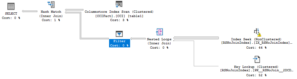
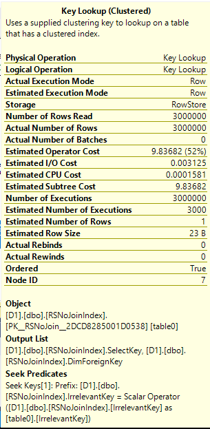
The plan has a total cost of 0.198516 optimizer units. If you know anything about row goals (this may be a good time for the reader to visit Paul White’s series on row goals) you might not be terribly surprised by the outcome. The row goal introduced by the TOP (1) makes the nested loop join very attractive in comparison to other plan choices. The cost of the scan on OUTER_HEAP is discounted from 2.93662 units to 0.0036173 units and the optimizer only expects to do 116 clustered index seeks against INNER_CI before it finds a row that does not match. However, we know our data and we know that all rows match. Therefore, the query will not return any rows and it must scan all rows in OUTER_HEAP if I execute the query. On my machine the query takes about two seconds:

CPU time = 1953 ms, elapsed time = 1963 ms.

If we’re going to read most of the rows anyway why not try a HASH JOIN hint? At least that plan won’t have a million clustered index seeks:a29_HJ_PLANThe new plan runs in MAXDOP 4 on my machine (although for not very long due to CPU cooling issues) and has a total cost of 19.9924 optimizer units. Query execution finishes in significantly less time:

CPU time = 1187 ms, elapsed time = 372 ms.

The Riddle


Can we do better than an ugly join hint? Microsoft blessed us with USE HINT functionality in SQL Server 2016 SP1, so let’s go ahead and try that to see if we can improve the performance of the query. To understand the full effect of the hint let’s get estimated plans for OPTION clauses of (USE HINT ('DISABLE_OPTIMIZER_ROWGOAL'), LOOP JOIN) and (USE HINT ('DISABLE_OPTIMIZER_ROWGOAL'), HASH JOIN). In theory, that will make it easy to compare the two queries:a29_compare_plans
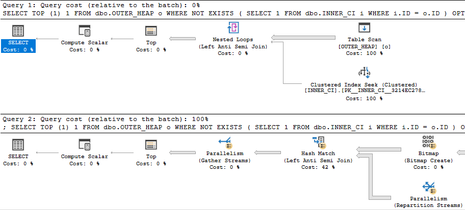
Something looks very wrong here. The loop join plan has a significantly lower cost than the hash join plan! In fact, the loop join plan has a total cost of 0.0167621 optimizer units. Why would disabling row goals for such a plan cause a decrease in total query cost?I uploaded the estimated plans here for those who wish to examine them without going through the trouble of creating tables.

Let’s Try Adding Trace Flags


First let’s try the query with just a USE HINT and no join hint. I get the hash join plan shape that I was after with a total cost of 19.9924 optimizer units. That’s definitely a good thing, but why did the optimizer pick that plan? The plan with a loop join is quite a bargain at 0.0167621 optimizer units. The optimization level is FULL, but that doesn’t mean that every possible plan choice was evaluated. Perhaps the answer is as simple as the optimizer did not consider a nested loop join plan while evaluating possible plan choices.There are a few different ways to see which optimizer rules were considered during query plan compilation. We can add trace flags 3604 and 8619 at the query level to get information about the rules that were applied during optimization. All of these trace flags are undocumented, don’t use them in production, blah blah blah. For clarity, the query now looks like this:

SELECT TOP (1) 1FROM dbo.OUTER_HEAP oWHERE NOT EXISTS(SELECT 1FROM dbo.INNER_CI iWHERE i.ID = o.ID) OPTION (USE HINT ('DISABLE_OPTIMIZER_ROWGOAL'), QUERYTRACEON 3604, QUERYTRACEON 8619);

Among other rules, we can see a few associated with nested loops:Apply Rule: LeftSideJNtoIdxLookup - LOJN/LSJ/LASJ -> IDX LOOKUPApply Rule: LASJNtoNL - LASJN -> NL

So the optimizer did consider nested loop joins at some point but it went with the hash join plan instead. That's interesting.

Let's Try More Trace Flags


A logical next step is to try to get more operator costing information. Perhaps the cost of the nested loop join plan when considered during optimization is different from the value displayed in the query plan in SSMS. As the optimizer applies different rules and does different transformations the overall cost can change, so I suppose this isn't a totally unreasonable theory. My first attempt at getting cost information for multiple plan options is by looking at the final memo for the query. This can be done with trace flag 8615.For clarity, the query now looks like this:

SELECT TOP (1) 1FROM dbo.OUTER_HEAP oWHERE NOT EXISTS(SELECT 1FROM dbo.INNER_CI iWHERE i.ID = o.ID) OPTION (USE HINT ('DISABLE_OPTIMIZER_ROWGOAL'), QUERYTRACEON 3604, QUERYTRACEON 8615-- , QUERYTRACEON 8619);

Group 8 is the only one with any costing information for joins:Group 8: Card=16935.2 (Max=1.1e+006, Min=0)11 PhyOp_HashJoinx_jtLeftAntiSemiJoin 6.9 7.10 5.0 Cost(RowGoal 0,ReW 0,ReB 0,Dist 0,Total 0)= 26.5569 (Distance = 1)4 PhyOp_HashJoinx_jtLeftAntiSemiJoin 6.4 7.3 5.0 Cost(RowGoal 0,ReW 0,ReB 0,Dist 0,Total 0)= 38.4812 (Distance = 1)1 LogOp_RightAntiSemiJoin 7 6 5 (Distance = 1)0 LogOp_LeftAntiSemiJoin 6 7 5 (Distance = 0)

This is rather disappointing. There's only costing information for a few hash join plans. We know that other join types were considered. Perhaps they were discarded from the memo. The final memo just doesn't have enough information to answer our question.

We Must Not Be Using Enough Trace Flags


There's a trace flag that adds memo arguments to trace flag 8619: 8620. Perhaps that will give us additional clues. For clarity, the query now looks like this:

SELECT TOP (1) 1FROM dbo.OUTER_HEAP oWHERE NOT EXISTS(SELECT 1FROM dbo.INNER_CI iWHERE i.ID = o.ID) OPTION (USE HINT ('DISABLE_OPTIMIZER_ROWGOAL'), QUERYTRACEON 3604, QUERYTRACEON 8615, QUERYTRACEON 8619, QUERYTRACEON 8620);

The output is again disappointing. I'll skip covering it and jump to trace flag 8621. That one adds additional information about the rules and how they interact with memos. With this trace flag we find more information about the plans with merge or loop joins:Rule Result: group=8 1 LogOp_RightAntiSemiJoin 7 6 5 (Distance = 1)Rule Result: group=8 2 PhyOp_MergeJoin 1-M x_jtRightAntiSemiJoin 7 6 5 (Distance = 2)Rule Result: group=8 3 PhyOp_HashJoinx_jtRightAntiSemiJoin 7 6 5 (Distance = 2)Rule Result: group=8 4 PhyOp_HashJoinx_jtLeftAntiSemiJoin 6 7 5 (Distance = 1)Rule Result: group=8 5 PhyOp_Applyx_jtLeftAntiSemiJoin 6 16 (Distance = 1)Rule Result: group=8 6 PhyOp_Applyx_jtLeftAntiSemiJoin 6 16 (Distance = 1)Rule Result: group=8 7 PhyOp_LoopsJoinx_jtLeftAntiSemiJoin 6 17 5 (Distance = 1)Rule Result: group=8 8 PhyOp_LoopsJoinx_jtLeftAntiSemiJoin 6 7 5 (Distance = 1)Rule Result: group=8 9 PhyOp_MergeJoin 1-M x_jtRightAntiSemiJoin 7 6 5 (Distance = 2)Rule Result: group=8 10 PhyOp_HashJoinx_jtRightAntiSemiJoin 7 6 5 (Distance = 2)Rule Result: group=8 11 PhyOp_HashJoinx_jtLeftAntiSemiJoin 6 7 5 (Distance = 1)Rule Result: group=8 12 PhyOp_Applyx_jtLeftAntiSemiJoin 6 16 (Distance = 1)Rule Result: group=8 13 PhyOp_Applyx_jtLeftAntiSemiJoin 6 16 (Distance = 1)Rule Result: group=8 14 PhyOp_LoopsJoinx_jtLeftAntiSemiJoin 6 17 5 (Distance = 1)Rule Result: group=8 15 PhyOp_LoopsJoinx_jtLeftAntiSemiJoin 6 17 5 (Distance = 1)Rule Result: group=8 16 PhyOp_LoopsJoinx_jtLeftAntiSemiJoin 6 7 5 (Distance = 1)Rule Result: group=8 17 PhyOp_LoopsJoinx_jtLeftAntiSemiJoin 6 7 5 (Distance = 1)

However, group 8 in the final memo still looks the same as before:Group 8: Card=16935.2 (Max=1.1e+006, Min=0)11 PhyOp_HashJoinx_jtLeftAntiSemiJoin 6.9 7.10 5.0 Cost(RowGoal 0,ReW 0,ReB 0,Dist 0,Total 0)= 26.5569 (Distance = 1)4 PhyOp_HashJoinx_jtLeftAntiSemiJoin 6.4 7.3 5.0 Cost(RowGoal 0,ReW 0,ReB 0,Dist 0,Total 0)= 38.4812 (Distance = 1)1 LogOp_RightAntiSemiJoin 7 6 5 (Distance = 1)0 LogOp_LeftAntiSemiJoin 6 7 5 (Distance = 0)

My interpretation is that costing information for the other join types was discarded from the memo. For example, at one point there was an item 5 in group 8 which contained information relevant to costing for one of the nested loop join plans. All of that information is not present in the final plan because the hash join plan was cheaper.

Pray to the Trace Flag Gods


There is an undisclosed trace flag which does not allow items to be discarded from the memo. Obviously this is a dangerous thing to do. However, with that trace flag group 8 finally reveals all of its secrets:Group 8: Card=16935.2 (Max=1.1e+006, Min=0)17 PhyOp_LoopsJoinx_jtLeftAntiSemiJoin 6 7 5.0 (Distance = 1)16 PhyOp_LoopsJoinx_jtLeftAntiSemiJoin 6 7 5.0 (Distance = 1)15 PhyOp_LoopsJoinx_jtLeftAntiSemiJoin 6 17 5.0 (Distance = 1)14 PhyOp_LoopsJoinx_jtLeftAntiSemiJoin 6 17 5.0 (Distance = 1)13 PhyOp_Applyx_jtLeftAntiSemiJoin 6 16 (Distance = 1)12 PhyOp_Applyx_jtLeftAntiSemiJoin 6 16 (Distance = 1)11 PhyOp_HashJoinx_jtLeftAntiSemiJoin 6.9 7.10 5.0 Cost(RowGoal 0,ReW 0,ReB 0,Dist 0,Total 0)= 26.5569 (Distance = 1)10 PhyOp_HashJoinx_jtRightAntiSemiJoin 7.8 6 5 (Distance = 2)9 PhyOp_MergeJoin 1-M x_jtRightAntiSemiJoin 7.6 6 5 (Distance = 2)8 PhyOp_LoopsJoinx_jtLeftAntiSemiJoin 6 7 5.0 (Distance = 1)7 PhyOp_LoopsJoinx_jtLeftAntiSemiJoin 6 17 5.0 (Distance = 1)6 PhyOp_Applyx_jtLeftAntiSemiJoin 6 16 (Distance = 1)5 PhyOp_Applyx_jtLeftAntiSemiJoin 6 16 (Distance = 1)4 PhyOp_HashJoinx_jtLeftAntiSemiJoin 6.4 7.3 5.0 Cost(RowGoal 0,ReW 0,ReB 0,Dist 0,Total 0)= 38.4812 (Distance = 1)3 PhyOp_HashJoinx_jtRightAntiSemiJoin 7.3 6.4 5.0 Cost(RowGoal 0,ReW 0,ReB 0,Dist 0,Total 0)= 48.5597 (Distance = 2)2 PhyOp_MergeJoin 1-M x_jtRightAntiSemiJoin 7.1 6.2 5.0 Cost(RowGoal 0,ReW 0,ReB 0,Dist 0,Total 0)= 106.564 (Distance = 2)1 LogOp_RightAntiSemiJoin 7 6 5 (Distance = 1)0 LogOp_LeftAntiSemiJoin 6 7 5 (Distance = 0)

Let's consider item 5 because it's one of the more reasonable loop join plan options. Item 5 doesn't give us direct costing information but it directs us to look to group 16:Group 16: Card=1 (Max=1, Min=0)2 PhyOp_Range 1 ASC 5.0 Cost(RowGoal 0,ReW 0,ReB 999999,Dist 1e+006,Total 1e+006)= 165.607 (Distance = 2)1 PhyOp_Range 1 ASC 5.0 Cost(RowGoal 0,ReW 0,ReB 999999,Dist 1e+006,Total 1e+006 s)= 165.607 (Distance = 2)0 LogOp_SelectIdx 15 5 (Distance = 1)

We can see a cost of 165.607 for the clustered index seeks on the inner side of the join. If that was the cost used when comparing plans then it explains why the optimizer opted for a hash join over the loop join. We might try looking at a query plan for the following:

DECLARE @TOP INT = 1;SELECT TOP (@TOP) 1FROM dbo.OUTER_HEAP oWHERE NOT EXISTS(SELECT 1FROM dbo.INNER_CI iWHERE i.ID = o.ID)OPTION (OPTIMIZE FOR (@TOP = 987654321), LOOP JOIN, MAXDOP 1);

With the above syntax we will get the same query results as before but the effective TOP (1) cannot change the cost of the query. Here are the operator details for the clustered index seek on INNER_CI:a29_seek_costs
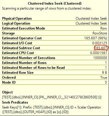
It's an exact match. The total cost of the query is 172.727 optimizer units, which is significantly more than the price tag of 19.9924 units for the hash join plan.

Improving Displayed Costing


So is there really a problem with the displayed cost of the plan with hints matching (USE HINT ('DISABLE_OPTIMIZER_ROWGOAL'), LOOP JOIN)? After all, the USE HINT seemed to give the correct plan shape without the join hints. Let's compare the TOP plan side by side with it:a29_compare_nl_plans
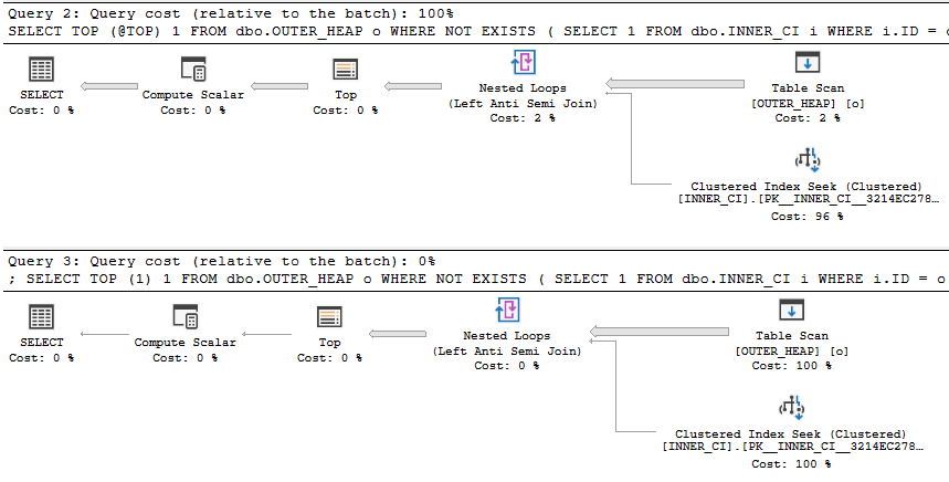
I also uploaded the estimated plans here.In my view, the costs of the USE HINT plan are nonsensical. The scan and the seeks have matching operator costs of 0.0167621 units. Bizarrely, this also matches the final query cost. 0.0167621 + 0.0167621 = 0.0167621. It's totally unclear where these numbers come from, and if a TOP (1) can aggressively discount all of the operators in a plan then it seems like the DISABLE_OPTIMIZER_ROWGOAL hint will not have its intended practical impact. Certainly a TOP (1) will not discount the costs of blocking operators, so plans without them (such as loop joins) will be costed cheaper than plans with them (like hash joins).I would prefer to see matching query costs for both subtrees. Of course, the TOP (1) can influence the costs of other parts of the plan that depend on this subtree, so the estimate needs to obey the TOP expression. I just feel that it shouldn't affect the cost of the immediate subtree.If you're curious where the 0.016762 number comes from, I suspect that it has something to do with the TOP (1) capping the cost of the nested loop join. The following can be found in the final memo:Group 11: Card=1 (Max=1, Min=0)1 PhyOp_Top 8.2 9.0 10.0 Cost(RowGoal 0,ReW 0,ReB 0,Dist 0,Total 0)= 0.016762 (Distance = 1)Group 8: Card=16935.2 (Max=1.1e+006, Min=0)2 PhyOp_Applyx_jtLeftAntiSemiJoin 6.4 15.2 Cost(RowGoal 0,ReW 0,ReB 0,Dist 0,Total 0)= 172.723 (Distance = 1)

In addition, the query cost slightly increases when I change the query to return the first 2 rows. You could argue that query plan costs are just numbers and there's no reason to care about them as long as you get the right plan, but that's not quite true. I'm sure this isn't an exhaustive list, but query plan costs can affect at least the following:

  • If the query cost is too low it won't be eligible for a parallel plan.
  • The number of seconds that a query will wait for a memory grant before throwing an error.
  • The amount of steps taken by the optimizer during query plan creation.
  • If the query is sent to a small query resource semaphore.
  • If the query is not able to run due to the query governor cost limit.

Final Thoughts


Congrats if you made it to the end.

Thanks for reading!

Going Further


If this is the kind of SQL Server stuff you love learning about, you'll love my training. I'm offering a 75% discount to my blog readers if you click from here. I'm also available for consulting if you just don't have time for that and need to solve performance problems quickly.

The Return of RESERVED_MEMORY_ALLOCATION_EXT

It is possible to see a scalability bottleneck in the form of high average wait time for the RESERVED_MEMORY_ALLOCATION_EXT wait if a highly concurrent workload is run on a server that consumes memory with batch mode operators. I believe that the severity of the bottleneck depends on unknown factors in the server’s initial memory state and the rate of memory actually used by queries to run batch mode operations. This blog post shares a reproduction of the issue along with a call to action.

The Test Query


Data prep for the test query is very simple. We throw the first ten million sequential integers into two single column BIGINT tables. Additionally, an empty CCI is created to add eligibility for batch mode as desired:

DROP TABLE IF EXISTS DUMMY_CCI;
CREATE TABLE DUMMY_CCI (
	ID INT,
	INDEX CCI CLUSTERED COLUMNSTORE
);

DROP TABLE IF EXISTS HASH_JOIN_SCALE_TEST_1;
CREATE TABLE HASH_JOIN_SCALE_TEST_1 (
	ID BIGINT NOT NULL
);

INSERT INTO HASH_JOIN_SCALE_TEST_1 WITH (TABLOCK)
SELECT TOP (10000000) ROW_NUMBER()
	OVER (ORDER BY (SELECT NULL))
FROM master..spt_values t1
CROSS JOIN master..spt_values t2
CROSS JOIN master..spt_values t3
OPTION (MAXDOP 1);

DROP TABLE IF EXISTS HASH_JOIN_SCALE_TEST_2;
CREATE TABLE HASH_JOIN_SCALE_TEST_2 (
ID BIGINT NOT NULL
);

INSERT INTO HASH_JOIN_SCALE_TEST_2 WITH (TABLOCK)
SELECT TOP (10000000) ROW_NUMBER()
	OVER (ORDER BY (SELECT NULL))
FROM master..spt_values t1
CROSS JOIN master..spt_values t2
CROSS JOIN master..spt_values t3
OPTION (MAXDOP 1);

The SELECT query that we’re going to test with joins them together and returns a count of distinct IDs:

SELECT COUNT(DISTINCT t1.ID)
FROM dbo.HASH_JOIN_SCALE_TEST_1 t1
LEFT OUTER JOIN dbo.HASH_JOIN_SCALE_TEST_2 t2
	ON t1.ID = t2.ID
OPTION (MAXDOP 1);

This is certainly an odd thing to do, but the point of this query is to create a simple test case that uses a bit of memory to create hash tables. Without any indexes on the table we’re very likely to get a hash join. In row mode the query takes about 17 seconds on the test server and uses 1257528 KB of memory.

As far as I can tell this query is a good fit for batch mode. The join is on BIGINT columns and everything except for the rowstore scans can execute in batch mode:

a28_query_plan

Even with the hidden conversions of 20 million rows from row mode to batch mode the query finishes in about 5 seconds. It uses significantly less memory compared to the row mode query: 386112 KB. All of this seems very reasonable.

Testing at Scale


The situation becomes less reasonable once there are many concurrent queries running at once. We go from the batch mode query running in a third of the time of row mode to sometimes running slower. Testing was done with 96 concurrent queries each running queries until 576 total queries were completed. Below is a graph of OS CPU and OS privileged time CPU based on perfmon data:

a28_cpu_graphs

The first third of the graph corresponds to the batch mode workload. CPU never hits 100% and is extremely variable during the run. We also see a high amount of privileged time in the OS. Within SQL Server, we use a total of 222,400,512 KB of query memory. The total wait time for RESERVED_MEMORY_ALLOCATION_EXT can vary, but for this one it was around 11.5 million ms.

The second third of the graph is the part that resets the server memory state. As stated in the introduction, this scalability bottleneck doesn’t always happen and seems to have some kind of dependency on the server’s initial memory state. Here we do a SELECT COUNT(*) on a 1 TB table to add pressure to the rowstore buffer pool.

The final third of the graph corresponds to the row mode workload. CPU jumps to near 100% very quickly and doesn’t waver much during the run. There is very little privileged time in the OS. Within SQL Server, we use a total of 724,336,128 KB of query memory. The wait time for RESERVED_MEMORY_ALLOCATION_EXT is always significantly reduced compared to batch mode. For this run it was around 107k ms.

In conclusion, we see about 1% of memory wait time with the row mode workload compared to the batch mode workload. Usually the row mode workload finishes a little faster than the batch mode one, despite needing over 3X as much total memory and the per-query efficiency advantage of batch mode.

Speculation on the Problem


There may be a hint in the memory management architecture guide:

Starting with SQL Server 2012, SQL Server might allocate more memory than the value specified in the max server memory setting. This behavior may occur when the Total Server Memory (KB) value has already reached the Target Server Memory (KB) setting (as specified by max server memory). If there is insufficient contiguous free memory to meet the demand of multi-page memory requests (more than 8 KB) because of memory fragmentation, SQL Server can perform over-commitment instead of rejecting the memory request.

This behavior is typically observed during the following operations: Large Columnstore index queries.

There are observable differences in how memory is allocated for the same operator when switching from batch mode to row mode. The number of wait events for RESERVED_MEMORY_ALLOCATION_EXT is significantly higher for row mode compared to batch mode. In addition, it remains nearly constant when TF 834 is enabled:

a28_memory_waits

TF 834 appears to fully resolve the scalability issue with batch mode, just like last time. It offers a dramatic improvement in workload completion time:

a28_summary_of_timings

Perhaps some batch mode operators require contiguous free memory for their allocations but the same operation done through row mode does not have that restriction. I can’t go any further than this because I don’t know anything about OS internals or memory management, but it could explain why we see such different behavior between row mode and batch mode.

Use Your Voice


Since SQL Server 2012, Microsoft has listed TF 834 as incompatible with columnstore. There are lots of scary consequences:

  • A non-yielding scheduler error and associated memory dumps in the SQL Server Error log.
  • Columnstore queries trigger severe performance issues.
  • A SQL Server instance triggers access violations when you execute Columnstore queries.
  • You encounter the following error when you run sp_createstats

However, I’ve been told that many of the SQL Server columnstore benchmarks for the TPC-H benchmarks use TF 834. It seems to be a natural fit for columnstore, and there are some workloads (seen in the lab and reproduced in the last two blog posts) where it resolves a key scalability bottleneck which is difficult to address through other means. I have created a feedback item on UserVoice requesting that Microsoft support TF 834 with columnstore.

Final Thoughts


Please provide feedback on the UserVoice item if you are able to do so. Thanks for reading!

Large Clustered Columnstore Index ETLs Cannot Scale Without TF 834 In SQL Server

Large servers may experience a scalability bottleneck related to the RESERVED_MEMORY_ALLOCATION_EXT wait event during loading of columnstore tables. This blog post shares a reproduction of the issue and discusses some test results.

The Test Server


Testing was done on a four socket bare metal server with 24 cores per socket. The server had 1 TB of RAM and storage was provided by a SAN. Within SQL Server, we were able to read data at a peak rate of about 5.5 GB/s. Hyperthreading was disabled, but there aren’t any other nonstandard OS configuration settings that I’m aware of.

SQL Server 2016 SP1 CU7 was installed on Windows Server 2016. Most default settings were retained for this testing, including allowing auto soft-NUMA to break up the 96 schedulers into 12 groups of 8, with 3 per memory node. Max server memory was set to around 800000 MB. The user database had 24 data files, indirect checkpoints weren’t used, and the memory model in use was conventional. No interesting trace flags were enabled, except perhaps for TF 4199. I did grow max server memory to close to the maximum before starting any of the tests.

Testing Code and Method


The workload test loaded the same data from a SQL Server table into 576 CCI target tables. For my testing I used a source table of one million rows. Each session grabs a number from a sequence, loads data into the table corresponding to the sequence number, and continues to do that until there are no more tables to process. This may seem like an odd test to run, but think of it as an abstract representation of a columnstore ETL workload which loads data into partitioned CCIs.

The first step is to define the source table. I created a 50 column table that stored only 0s in all of its rows. There’s nothing particularly special about this choice other that it has a very low disk footprint as a CCI because it compresses so well. On a non-busy system it took around 7.3 seconds to insert one million rows into a CCI. Below is the table definition:

DROP TABLE IF EXISTS CCI_SOURCE;

CREATE TABLE CCI_SOURCE (
ID1 SMALLINT,
ID2 SMALLINT,
ID3 SMALLINT,
ID4 SMALLINT,
ID5 SMALLINT,
ID6 SMALLINT,
ID7 SMALLINT,
ID8 SMALLINT,
ID9 SMALLINT,
ID10 SMALLINT,
ID11 SMALLINT,
ID12 SMALLINT,
ID13 SMALLINT,
ID14 SMALLINT,
ID15 SMALLINT,
ID16 SMALLINT,
ID17 SMALLINT,
ID18 SMALLINT,
ID19 SMALLINT,
ID20 SMALLINT,
ID21 SMALLINT,
ID22 SMALLINT,
ID23 SMALLINT,
ID24 SMALLINT,
ID25 SMALLINT,
ID26 SMALLINT,
ID27 SMALLINT,
ID28 SMALLINT,
ID29 SMALLINT,
ID30 SMALLINT,
ID31 SMALLINT,
ID32 SMALLINT,
ID33 SMALLINT,
ID34 SMALLINT,
ID35 SMALLINT,
ID36 SMALLINT,
ID37 SMALLINT,
ID38 SMALLINT,
ID39 SMALLINT,
ID40 SMALLINT,
ID41 SMALLINT,
ID42 SMALLINT,
ID43 SMALLINT,
ID44 SMALLINT,
ID45 SMALLINT,
ID46 SMALLINT,
ID47 SMALLINT,
ID48 SMALLINT,
ID49 SMALLINT,
ID50 SMALLINT
);

INSERT INTO CCI_SOURCE WITH (TABLOCK)
SELECT
 ID,ID,ID,ID,ID,ID,ID,ID,ID,ID
,ID,ID,ID,ID,ID,ID,ID,ID,ID,ID
FROM (
	SELECT TOP (1000000) 0 ID
	FROM master..spt_values t1
	CROSS JOIN master..spt_values t2
) t;

Next we need a stored procedure that can save off previous test results (as desired) and reset the server for the next test. If a test name is passed in then results are saved to CCI_TEST_RESULTS and CCI_TEST_WAIT_STATS from the previous run. The procedure always recreates all of the target CCI tables, resets the sequence, clears the buffer pool, and does a few other things.

CREATE OR ALTER PROCEDURE [dbo].[CCI_TEST_RESET] (@PreviousTestName NVARCHAR(100) = NULL, @DebugMe INT = 0)
AS
BEGIN
	DECLARE
	@tablename SYSNAME,
	@table_number INT = 1,
	@SQLToExecute NVARCHAR(4000);

	/*
CREATE TABLE CCI_TEST_WAIT_STATS (
	TEST_NAME NVARCHAR(100),
	WAIT_TYPE NVARCHAR(60),
	WAITING_TASKS_COUNT BIGINT,
	WAIT_TIME_MS BIGINT,
	MAX_WAIT_TIME_MS BIGINT,
	SIGNAL_WAIT_TIME_MS BIGINT
);

CREATE TABLE CCI_TEST_RESULTS (
	TEST_NAME NVARCHAR(100),
	TOTAL_SESSION_COUNT SMALLINT,
	TEST_DURATION INT,
	TOTAL_WORK_TIME INT,
	BEST_TABLE_TIME INT,
	WORST_TABLE_TIME INT,
	TOTAL_TABLES_PROCESSED SMALLINT,
	MIN_TABLES_PROCESSED SMALLINT,
	MAX_TABLES_PROCESSED SMALLINT
);
	*/

	SET NOCOUNT ON;

	IF @DebugMe = 0
	BEGIN
		DROP SEQUENCE IF EXISTS CCI_PARALLEL_TEST_SEQ;
		CREATE SEQUENCE CCI_PARALLEL_TEST_SEQ
			AS SMALLINT
			START WITH 1
			INCREMENT BY 1
			CACHE 600;

		IF @PreviousTestName  N''
		BEGIN
			INSERT INTO CCI_TEST_RESULTS WITH (TABLOCK)
			SELECT @PreviousTestName,
			  COUNT(*) TOTAL_SESSION_COUNT
			, DATEDIFF(MILLISECOND, MIN(MIN_START_TIME), MAX(MAX_END_TIME)) TEST_DURATION
			, SUM(TOTAL_SESSION_TIME) TOTAL_WORK_TIME
			, MIN(MIN_TABLE_TIME) BEST_TABLE_TIME
			, MAX(MAX_TABLE_TABLE) WORST_TABLE_TIME
			, SUM(CNT) TOTAL_TABLES_PROCESSED
			, MIN(CNT) MIN_TABLES_PROCESSED
			, MAX(CNT) MAX_TABLES_PROCESSED
			FROM (
				SELECT
				  SESSION_ID
				, COUNT(*) CNT
				, SUM(DATEDIFF(MILLISECOND, START_TIME, END_TIME)) TOTAL_SESSION_TIME
				, MIN(DATEDIFF(MILLISECOND, START_TIME, END_TIME)) MIN_TABLE_TIME
				, MAX(DATEDIFF(MILLISECOND, START_TIME, END_TIME)) MAX_TABLE_TABLE
				, MIN(START_TIME) MIN_START_TIME
				, MAX(END_TIME) MAX_END_TIME
				FROM CCI_TEST_LOGGING_TABLE
				GROUP BY SESSION_ID
			) t;

			INSERT INTO CCI_TEST_WAIT_STATS WITH (TABLOCK)
			SELECT @PreviousTestName, * FROM sys.dm_os_wait_stats
			WHERE wait_type IN (
				'RESERVED_MEMORY_ALLOCATION_EXT'
				, 'SOS_SCHEDULER_YIELD'
				, 'PAGEIOLATCH_EX'
				, 'MEMORY_ALLOCATION_EXT'
				, 'PAGELATCH_UP'
				, 'PAGEIOLATCH_SH'
				, 'WRITELOG'
				, 'LATCH_EX'
				, 'PAGELATCH_EX'
				, 'PAGELATCH_SH'
				, 'CMEMTHREAD'
				, 'LATCH_SH'
			);

		END;

		DROP TABLE IF EXISTS CCI_TEST_LOGGING_TABLE;
		CREATE TABLE CCI_TEST_LOGGING_TABLE (
			SESSION_ID INT,
			TABLE_NUMBER INT,
			START_TIME DATETIME,
			END_TIME DATETIME
		);

	END;

	WHILE @table_number BETWEEN 0 AND 576
	BEGIN
		SET @tablename = N'CCI_PARALLEL_RPT_TARGET_' + CAST(@table_number AS NVARCHAR(3));
		SET @SQLToExecute= N'DROP TABLE IF EXISTS ' + QUOTENAME(@tablename);
		IF @DebugMe = 1
		BEGIN
			PRINT @SQLToExecute;
		END
		ELSE
		BEGIN
			EXEC (@SQLToExecute);
		END;

		SET @SQLToExecute = N'SELECT * INTO ' + QUOTENAME(@tablename) +
		' FROM CCI_SOURCE WHERE 1 = 0';
		IF @DebugMe = 1
		BEGIN
			PRINT @SQLToExecute;
		END
		ELSE
		BEGIN
			EXEC (@SQLToExecute);
		END;

		SET @SQLToExecute = N'CREATE CLUSTERED COLUMNSTORE INDEX CCI ON ' + QUOTENAME(@tablename);
		IF @DebugMe = 1
		BEGIN
			PRINT @SQLToExecute;
		END
		ELSE
		BEGIN
			EXEC (@SQLToExecute);
		END;

		SET @table_number = @table_number + 1;
	END;

	IF @DebugMe = 0
	BEGIN
		DBCC DROPCLEANBUFFERS WITH NO_INFOMSGS;
		DBCC FREEPROCCACHE WITH NO_INFOMSGS;
		DBCC FREESYSTEMCACHE('ALL');

		SELECT COUNT(*) FROM CCI_SOURCE; -- read into cache

		DBCC SQLPERF ("sys.dm_os_wait_stats", CLEAR) WITH NO_INFOMSGS;
		DBCC SQLPERF ("sys.dm_os_spinlock_stats", CLEAR) WITH NO_INFOMSGS;
	END;
END;

Finally we need a stored procedure that can be called to do as many CCI inserts as it can as quickly as possible. I used the following code:

CREATE OR ALTER PROCEDURE [dbo].[CCI_RUN_INSERTS] (@DebugMe INT = 0)
AS
BEGIN
	DECLARE @table_number INT,
	@tablename SYSNAME,
	@SQLToExecute NVARCHAR(4000),
	@start_loop_time DATETIME;

	SET NOCOUNT ON;

	SELECT @table_number = NEXT VALUE FOR CCI_PARALLEL_TEST_SEQ;

	WHILE @table_number BETWEEN 0 AND 576
	BEGIN
		SET @start_loop_time = GETDATE();

		SET @tablename = N'CCI_PARALLEL_RPT_TARGET_' + CAST(@table_number AS NVARCHAR(3));
		SET @SQLToExecute= N'
		INSERT INTO ' + QUOTENAME(@tablename) + N' WITH (TABLOCK)
		SELECT * FROM CCI_SOURCE WITH (TABLOCK)
		OPTION (MAXDOP 1)';

		IF @DebugMe = 1
		BEGIN
			PRINT @SQLToExecute;
		END
		ELSE
		BEGIN
			EXEC (@SQLToExecute);

			INSERT INTO CCI_TEST_LOGGING_TABLE VALUES (@@SPID, @table_number, @start_loop_time, GETDATE());
		END;

		SELECT @table_number = NEXT VALUE FOR CCI_PARALLEL_TEST_SEQ;
	END;
END;

To vary the number of concurrent queries I used sqlcmd. Each set of 12 sessions had the following format:


START /B sqlcmd -d your_db_name -S your_server_name -Q "EXEC dbo.[CCI_RUN_INSERTS]" > nul
ping 192.2.0.1 -n 1 -w 1 > nul

My workflow was to perform this test was to add the desired number of calls to the stored procedure in the .bat file, run the test, and to check the results to make sure that the test was a good one. If it was I saved off results using the reset procedure. If not I ran the reset procedure and tried again.

The ping command is there to add a small delay between sets of queries. I found that adding such a delay led to less doubling up on schedulers. I picked 12 because that's the number of soft-NUMA nodes. Sometimes tests would get quite a bit of SOS_SCHEDULER_YIELD waits which would mean that they couldn't be accurately compared to other tests. My fix was to just run the test again. It required a bit of patience but I never had to run a test more than once. SOS waits weren't eliminated but I'd say they fell to acceptable levels:

a27_SOS_CPU_wait_table

The right way to avoid SOS waits for testing like this (which might require every user session to go on its own scheduler) would be to set up 96 manual soft-NUMA nodes. But who has time for that?

Test Results


12 tests with different numbers of active queries were run. I picked numbers that somewhat evenly divided into 576 to try to keep work balanced between threads. The blue line in the chart below measures how long each test took from start to finish and the orange line represents how fast the test could have completed if there was no contention on the server whatsoever:

thread count comparison

Naturally we can't expect the two lines to match perfectly, but improvements in runtime stop after going past 32 threads. In fact, the workload takes longer with 96 threads compared to 32 threads.

The dominant wait event for the higher thread count runs is RESERVED_MEMORY_ALLOCATION_EXT. Below is a chart of all of the wait events worth mentioning for the 96 thread run:

SQL Server wait stats
waiting, waiting

The total number of wait events for RESERVED_MEMORY_ALLOCATION_EXT is very consistent between runs. However, the average wait time significantly increases as the number of concurrent queries increases:

SQL Server Thread Counts
threads going up

In fact, it could be said that that nearly all worker time past 32 threads is spent waiting on memory. The final column in the chart below is the total time spent in SQL Server minus wait time for RESERVED_MEMORY_ALLOCATION_EXT. The values in that column are remarkably consistent.

SQL Server query runtimes
running wild

In my experience, when we get into a situation with high memory waits caused by too much concurrent CCI activity all queries on the server that use a memory grant can be affected. For example, I've seen sp_whoisactive run for longer than 90 seconds.

It needs to be stated that not all CCIs will suffer from this scalability problem. I was able to achieve good scalability with some artificial tables, but all of the real target tables that I tested have excessive memory waits at high concurrency. Perhaps tables which require more CPU to compress naturally spread out their memory requests and the underlying OS is better able to keep up.

Test Results With Trace Flag 834


Microsoft strongly recommends against using trace flag 834 with columnstore tables. There's even an article dedicated to that warning. I was desperate so I tried it anyway. The difference was night and day:

SQL Server Thread Count
trending

Enabling trace flag 834 does at least three things: SQL Server grows to max server memory on startup, AWE memory is used for memory access, and large pages are used for the buffer pool. I didn't see gains when using LPIM (which uses AWE memory) or by growing memory to max before running tests with a conventional memory model, so I suspect that the large pages are making a key difference. Wait time for RESERVED_MEMORY_ALLOCATION_EXT is under a second for all tests.

Scalability is diminished a bit for the 96 thread run. There are some wait events that creep up:

SQL Server Wait Times
bigwaits4u

All of the wait events can be troubleshooted in conventional ways except possibly for CMEMTHREAD. There's no longer a large amount of time spent outside of SQL Server in the OS.

Other Workarounds


Without trace flag 834 this can be a difficult problem to work around. The two main strategies are to spread out CCI insert activity as much as possible during the ETL and to reduce memory usage of queries which run at the same time as the CCI inserts. For example, consider a query that inserts into a CCI that also performs a large hash join. If that hash join can be moved to somewhere else in the process then you might come out ahead in reducing contention on memory.

Other than that, there's some evidence that virtualized servers are not a good fit for this type of workload. Large virtual guests experience the memory waits at an increased rate, but it isn't yet clear if the problem can be avoided through some change in VM configuration.

Final Thoughts


It's hard not to conclude that TF 834 is necessary to get scalability for columnstore ETLs on very large servers. Hopefully Microsoft will make TF 834 compatible with columnstore one day in the future.

Thanks for reading!

Going Further


If this is the kind of SQL Server stuff you love learning about, you'll love my training. I'm offering a 75% discount to my blog readers if you click from here. I'm also available for consulting if you just don't have time for that and need to solve performance problems quickly.

Batch Mode Memory Fractions In SQL Server Query Plans

My least favorite tempdb spills are the ones that happen with a large percentage of the memory grant remaining unused. For example, recently I saw tempdb spills with a memory grant of 35 GB but SQL Server reported that only 10 GB of memory was used. Usually this problem can be traced back to suboptimal memory fractions somewhere in a query plan. I suspect that it can also happen with certain types of queries that load data into columnstore tables but haven’t verified that. In the test environment the issue was caused by memory fractions, but these memory fractions were attached to batch mode operators. The rules for batch mode memory fractions certainly appear to be different than those for rowstore memory fractions. I believe that I was able to work out a few of the details for a few simple cases. In some scenarios, plans with multiple batch mode hash joins can ask for significantly more memory than needed. Reducing the memory grant via Resource Governor or a query hint to something more reasonable can lead to unnecessary (and often frustrating) tempdb spills.

What is a Memory Fraction?


There’s very little information out there about memory fractions. I would define them as information in the query plan that can give you clues about each operator’s share of the total query memory grant. This is naturally more complicated for query plans that insert into tables with columnstore indexes but that won’t be covered here. Most references will tell you not to worry about memory fractions or that they aren’t useful most of the time. Out of thousands of queries that I’ve tuned I can only think of a few for which memory fractions were relevant. Sometimes queries spill to tempdb even though SQL Server reports that a lot of query memory was unused. In these situations I generally hope for a poor cardinality estimate which leads to a memory fraction which is too low for the spilling operator. If fixing the cardinality estimate doesn’t prevent the spill then things can get a lot more complicated, assuming that you don’t just give up.

Types of Query Plans


The demos for this blog post all use tables with identical structures and data. The tables are heaps so the plans will only feature hash joins. The most important plan characteristic is how many of the hash tables need to be kept in memory concurrently while the query processor executes the query. This is where memory fractions come in. The query optimizer tries to reuse parts of memory grants as it can. For example, if the hash build for the first join isn’t needed when the third join executes then it’s possible to use the memory grant from the first hash table for the third hash table. Some of the examples below will make this more clear.

The first type of plan has hash joins which can all run concurrently. Memory for the hash tables cannot be reused between operators.

SQL Server Query Plan
bushy

For that query, the MF_DEMO_1 table is the probe side for all of the joins. SQL Server builds all of the hash joins and then rows flow from the probe side through the plan (as long as there aren’t tempdb spills). I will refer to this type of plan as a “concurrent join plan” which is a term that I just made up.

The second type of plan has hash joins which cannot all run concurrently. Pairs of hash tables are active at the same time, but memory grants can be reused between operators.

SQL Server Query Plans
not bushy

For that query, the MF_DEMO_1 table is the build side for all of the joins. Each hash table blocks the next one from starting. This means that at most two hash tables need to be kept in memory at the same time. Query memory cannot be reused for joins 1 and 2 but join 3 can reuse memory from join 1 and join 4 can reuse memory from join 2. I will refer to this type of plan as a “nonconcurrent join plan” which is another term that I just made up.

If the above wasn’t clear I recommend running through the demos with live query statistics enabled. It can be very useful to understand how rows flow through a plan. As far as I know, all queries of this type can be implemented with the nonconcurrent pattern but not all queries can be implemented with the concurrent pattern .

Create the Tables


The table definitions for our demos are pretty boring. I’m using a VARCHAR(100) as the join column to blow up memory grants and requirements a bit. All of the tables are heaps and have about 6.5 million rows in them. TARGET_TABLE is used as a dumping ground for the inserts and #ADD_BATCH_MODE is used to switch the hash joins to batch mode as desired. All testing was done on SQL Server 2016 SP1 CU7.

DROP TABLE IF EXISTS MF_DEMO_1;
CREATE TABLE MF_DEMO_1 (
       ID VARCHAR(100)
);

INSERT INTO MF_DEMO_1 WITH (TABLOCK)
SELECT 999999999999999 + ROW_NUMBER()
	OVER (ORDER BY (SELECT NULL))
FROM master..spt_values t1
CROSS JOIN master..spt_values t2;

CREATE STATISTICS S1 ON MF_DEMO_1 (ID) WITH FULLSCAN;

DROP TABLE IF EXISTS MF_DEMO_2;
CREATE TABLE MF_DEMO_2 (
       ID VARCHAR(100)
);

INSERT INTO MF_DEMO_2 WITH (TABLOCK)
SELECT 999999999999999 + ROW_NUMBER()
	OVER (ORDER BY (SELECT NULL))
FROM master..spt_values t1
CROSS JOIN master..spt_values t2;

CREATE STATISTICS S2 ON MF_DEMO_2 (ID) WITH FULLSCAN;

DROP TABLE IF EXISTS MF_DEMO_3;
CREATE TABLE MF_DEMO_3 (
       ID VARCHAR(100)
); 

INSERT INTO MF_DEMO_3 WITH (TABLOCK)
SELECT 999999999999999 + ROW_NUMBER()
	OVER (ORDER BY (SELECT NULL))
FROM master..spt_values t1
CROSS JOIN master..spt_values t2;

CREATE STATISTICS S3 ON MF_DEMO_3 (ID) WITH FULLSCAN;

DROP TABLE IF EXISTS MF_DEMO_4;
CREATE TABLE MF_DEMO_4 (
       ID VARCHAR(100)
); 

INSERT INTO MF_DEMO_4 WITH (TABLOCK)
SELECT 999999999999999 + ROW_NUMBER()
	OVER (ORDER BY (SELECT NULL))
FROM master..spt_values t1
CROSS JOIN master..spt_values t2;

CREATE STATISTICS S4 ON MF_DEMO_4 (ID) WITH FULLSCAN;

DROP TABLE IF EXISTS MF_DEMO_5;
CREATE TABLE MF_DEMO_5 (
	ID VARCHAR(100)
); 

INSERT INTO MF_DEMO_5 WITH (TABLOCK)
SELECT 999999999999999 + ROW_NUMBER()
	OVER (ORDER BY (SELECT NULL))
FROM master..spt_values t1
CROSS JOIN master..spt_values t2;

CREATE STATISTICS S5 ON MF_DEMO_5 (ID) WITH FULLSCAN;

CREATE TABLE #ADD_BATCH_MODE (I INT, INDEX CCI CLUSTERED COLUMNSTORE);

DROP TABLE IF EXISTS TARGET_TABLE;

CREATE TABLE TARGET_TABLE (ID VARCHAR(100));

Row Mode Memory Fractions For Concurrent Join Plans


The following query results in a concurrent join plan with row mode hash joins:

INSERT INTO TARGET_TABLE WITH (TABLOCK)
SELECT t1.ID
FROM MF_DEMO_3 t3
RIGHT OUTER JOIN MF_DEMO_2 t2
RIGHT OUTER JOIN MF_DEMO_1 t1
ON t1.ID = t2.ID
ON t1.ID = t3.ID
OPTION (FORCE ORDER, MAXDOP 1);

The desired memory grant is 2860640 KB. The memory fractions for both join operators have an input of 0.5 and an output of 0.5. This is exactly as expected. The hash tables can both start at the same time and cannot reuse memory, so each operator gets 50% of the query memory grant for the plan. Adding a third join to the plan increases the query memory grant to 4290960 KB.

INSERT INTO TARGET_TABLE WITH (TABLOCK)
SELECT t1.ID
FROM MF_DEMO_4 t4
RIGHT OUTER JOIN MF_DEMO_3 t3
RIGHT OUTER JOIN MF_DEMO_2 t2
RIGHT OUTER JOIN MF_DEMO_1 t1
ON t1.ID = t2.ID
ON t1.ID = t3.ID
ON t1.ID = t4.ID
OPTION (FORCE ORDER, MAXDOP 1);

Again, this seems very reasonable. SQL Server now tries to builds three hash tables in memory at the same time. The memory fractions for each operator have fallen to 0.3333333. Each operator gets a third of the query memory grant.

Row Mode Memory Fractions For Nonconcurrent Join Plans


The following query results in a nonconcurrent join plan with row mode hash joins:

INSERT INTO TARGET_TABLE WITH (TABLOCK)
SELECT t1.ID
FROM MF_DEMO_1 t1
INNER JOIN MF_DEMO_2 t2 ON t1.ID = t2.ID
INNER JOIN MF_DEMO_3 t3 ON t2.ID = t3.ID
INNER JOIN MF_DEMO_4 t4 ON t3.ID = t4.ID
OPTION (MAXDOP 1, FORCE ORDER);

The query plan was uploaded here. I recommend downloading the all of the plans referenced in this blost post if you’re interested in them so you can see all of the details.

Here are the memory fractions for the rightmost join (node 3):

Memory Fractions Input: 1, Memory Fractions Output: 0.476174

here are the memory fractions for the middle join (node 2):

Memory Fractions Input: 0.523826, Memory Fractions Output: 0.5

and here are the memory fractions for the leftmost join (node 1):

Memory Fractions Input: 0.5, Memory Fractions Output: 1

What do all of those numbers mean? The rightmost join builds its hash table first and starts with all query memory available to it. However, the output fraction is 0.476174. That means that the hash table can only use up to 47.6% of the query memory granted to the plan. The middle join is able to use up to 50% (the minimum of the input and output fractions for the node) of the memory granted to the plan. Note that 0.476174 + 0.523826 = 1.0. The last join to start executing is also able to use up to 50% of the granted memory. That join is the last operator that uses memory in the plan so the output fraction is 1.0. Memory grant reuse allows the plan to use up to 147.6% of the memory grant over the lifetime of the query execution. Without memory grant reuse each operator wouldn’t be able to use as much memory.

Removing one of the joins results in the desired query memory grant dropping from 3146704 KB to 3003672 KB. This is a significantly less drop than the other query. The smaller decrease is expected because the third join that we added can reuse the memory grant from the first. As more joins are added to a nonconcurrent plan the desired memory grant grows at a much slower rate than the memory grant for the concurrent join plan.

Batch Mode Memory Fractions For Concurrent Join Plans


The query plan for the next query is somewhat dependent on hardware. On my machine I had to let it run in parallel to get batch mode hash joins:

INSERT INTO TARGET_TABLE WITH (TABLOCK)
SELECT t1.ID
FROM MF_DEMO_5 t5
RIGHT OUTER JOIN MF_DEMO_4 t4
RIGHT OUTER JOIN MF_DEMO_3 t3
RIGHT OUTER JOIN MF_DEMO_2 t2
RIGHT OUTER JOIN MF_DEMO_1 t1
LEFT OUTER JOIN #ADD_BATCH_MODE ON 1 = 0
ON t1.ID = t2.ID
ON t1.ID = t3.ID
ON t1.ID = t4.ID
ON t1.ID = t5.ID
OPTION (FORCE ORDER, MAXDOP 4);

The estimated plan is here. It’s easy to tell if the query is using batch mode joins because the joins are run in parallel but there are no repartition stream operators.

SQL Server Query Plan
parallel and bushy

SQL Server is not able to reuse memory grants for this query. SQL Server tries to build all of the hash tables in memory before probe side is processed. However, the memory fractions are different from before: 0.25, 0.5, 0.75, and 1.0. These memory fractions do not make sense if interpreted in the same way as before. How can the final hash join in the plan have an input memory fraction of 1.0?

It’s unclear what the memory fractions are supposed to mean here, but there is one observable difference compared to the row mode plan. In the row mode equivalent plan SQL Server divides the memory evenly between operators. For our very simple test plan this means that all of the hash joins will spill to tempdb or none of them will spill. Reducing a MAX_GRANT_PERCENT hint from the right value by 1% results in two spills:

SQL Server Query Plan
spilly

Both operators spilled because memory was divided evenly and there wasn’t enough memory to hold both hash tables in memory. However, with batch mode hash joins we can get plans like the following:

SQL Server Query Plan
spilly

How is it possible that one join spills but the other doesn’t? It is only possible if memory isn’t divided evenly. It appears that memory is used as needed in some situations. Unfortunately, the actual plan for batch mode operators doesn’t give us a lot of spill information like it does for row mode. There’s a debug channel extended event query_execution_batch_hash_join_spilled that can give us some clues. 657920 KB of memory was granted for a two batch mode hash join query. For the operator that spilled, only 44852457 bytes were written to memory on the build side. That’s about 43800 KB, which is significantly less than half of available query memory.

SQL Server Extended Events
spills!

We can’t conclude that exactly 44852457 bytes of memory were granted to the operator. However, it should be somewhat close. In conclusion, for these types of queries it isn’t clear what the memory grant fractions are supposed to mean. SQL Server is able to exceed them in some cases. It’s possible to see 0 bytes of memory used for the build side in the extended event. I believe that this is the bad type of memory reuse as opposed to the good kind.

Batch Mode Memory Fractions For Nonconcurrent Join Plans


The following query results in a nonconcurrent batch mode hash join plan on my machine:

INSERT INTO TARGET_TABLE WITH (TABLOCK)
SELECT t1.ID
FROM MF_DEMO_1 t1
LEFT OUTER JOIN #ADD_BATCH_MODE On 1 = 0
WHERE EXISTS (
	SELECT 1
	FROM MF_DEMO_2 t2 WHERE t1.ID = t2.ID
) AND EXISTS (
	SELECT 1
	FROM MF_DEMO_3 t3 WHERE t1.ID = t3.ID
) AND EXISTS (
	SELECT 1
	FROM MF_DEMO_4 t4 WHERE t1.ID = t4.ID
) AND EXISTS (
	SELECT 1
	FROM MF_DEMO_5 t5 WHERE t1.ID = t5.ID
) OPTION (MAXDOP 4, FORCE ORDER);

As far as I know there’s nothing special about the semijoins. I used them to keep the estimated row size as consistent as possible. The behavior detailed below can be observed with normal joins as well.

Here is the estimated query plan. The same memory fraction pattern of 0.25, 0.50, 0.75, and 1.00 can be found in this query. Based on the query’s structure, memory grant reuse should be allowed between operators. Alarmingly, this query has the same desired memory grant as one with four concurrent joins. The desired memory grant changes significantly as tables are added or removed. This is a big change in behavior compared to row mode batch joins.

As far as I can tell, memory grant reuse can happen in plans like this with batch mode hash joins. Removing or adding joins results in very small adjustments in maximum memory used during query execution. Still, it seems as if the query optimizer is assuming that memory cannot be reused. With this query pattern, the first operator to run does not have access more memory implied by the memory fraction. In fact, it has access to less memory implied by the memory fraction.

Running the query without any memory grant hints results in no tempdb spills and a maximum memory use of 647168 KB. Restricting the memory grant to 2 GB results in a tempdb spill for the rightmost operator. This is unexpected. 500000 KB of memory should be more than enough memory to avoid a spill. As before, the only way I could find to investigate this further was to use the query_execution_batch_hash_join_spilled extended event and to force tempdb spills using the MAX_GRANT_PERCENT query hint.

A good amount of testing suggested that the available memory per operator is the input memory fraction for that operator divided by the sum of all output memory fractions. The rightmost operator only gets 0.25 / (0.25 + 0.5 + 0.75 + 1.0) = 10% of the memory granted to the query, the next operator gets 20%, the next operator gets 30%, and the final operator gets 40%. The situation gets worse as more joins are added to the query. Keep in mind that we aren’t doing anything tricky with cardinality estimates or data types which would result in skewed estimates. The query optimizer seems to recognize that each join will require the same amount of memory for each hash join, but it doesn’t make the same minimum amount available for each operator. That’s what is so puzzling.

The preceding paragraph seems to contradict the idea that memory grant reuse is possible for these plan shapes. Perhaps for these simple plans memory grant reuse is possible but it cannot go above 100% like we saw in the row mode plan. This could still be helpful in that the query could steal less memory from the buffer pool, but it’s certainly not as helpful in avoiding spills as the behavior we get with the row mode plan. Under the assumption the total memory grants seem a bit more reasonable, although it’s hard not to object as to how SQL Server is distributing the memory to each operator.

We can avoid the spill by giving SQL Server the memory that it required, but this is undesirable if multiple concurrent queries are running. I’ve often observed higher than expected memory grants for queries with batch mode hash joins. An assumption that query memory reuse will not be available for batch mode hash joins can explain part of what I’ve observed. If memory grants are left unchecked, applications may see decreased possible concurrency due to RESOURCE_SEMAPHORE waits. Lowering memory grants through any available method can result in unnecessary (based on total memory granted) tempdb spills. It’s easy to get stuck between a rock and a hard place.

Batch Mode Workarounds


There is some hope for nonconcurrent batch mode hash join plans. SQL Server 2017 introduces adaptive memory feedback for these operators. I imagine that functionality is a poor fit for ETL queries which may process dramatically different amounts of data each day, so I can’t view it as a complete solution. It certainly doesn’t help us on SQL Server 2016. Are there workarounds to prevent spills without requiring excessive memory grants? Yes, but they are very ugly and I can only imagine using them when truly needed during something like an ETL process.

Consider the following query:

INSERT INTO TARGET_TABLE WITH (TABLOCK)
SELECT t1.ID
FROM MF_DEMO_1 t1
LEFT OUTER JOIN MF_DEMO_2 t2 ON t2.ID = t1.ID
LEFT OUTER JOIN MF_DEMO_3 t3 ON t3.ID = t2.ID
LEFT OUTER JOIN MF_DEMO_4 t4 ON t4.ID = t3.ID
LEFT OUTER JOIN MF_DEMO_4 t5 ON t5.ID = t4.ID
LEFT OUTER JOIN #ADD_BATCH_MODE ON 1 = 0
OPTION (FORCE ORDER, MAXDOP 4, MAX_GRANT_PERCENT = 60);

On my machine, the memory hint results in a memory grant of 2193072 KB. The rightmost join spills even when only a maximum of 1232896 KB of memory is used during query execution:

SQL Server Query Plan
more spills!

One way to avoid the spill is to shift the memory fractions in our favor. Ideally SQL Server would think that the rightmost join would need much more memory for its hash table than the other joins. If we can add an always NULL column with a large data type that is only needed for the first hash table, that might do the trick. The query syntax below isn’t guaranteed to get the plan that we want but it seems to work in this case:

ALTER TABLE MF_DEMO_1 ADD DUMMY_COLUMN_V4000 VARCHAR(4000) NULL;
ALTER TABLE MF_DEMO_2 ADD DUMMY_COLUMN_V10 VARCHAR(10) NULL;

INSERT INTO TARGET_TABLE WITH (TABLOCK)
SELECT t1.ID
FROM MF_DEMO_1 t1
LEFT OUTER JOIN MF_DEMO_2 t2 ON t2.ID = t1.ID
LEFT OUTER JOIN MF_DEMO_3 t3 ON t3.ID = t2.ID
LEFT OUTER JOIN MF_DEMO_4 t4 ON t4.ID = t3.ID
LEFT OUTER JOIN MF_DEMO_4 t5 ON t5.ID = t4.ID
LEFT OUTER JOIN #ADD_BATCH_MODE ON 1 = 0
WHERE (t1.DUMMY_COLUMN_V4000 IS NULL OR t2.DUMMY_COLUMN_V10 IS NULL)
OPTION (FORCE ORDER, MAXDOP 4, MAX_GRANT_PERCENT = 32);

An actual plan was uploaded here. The query no longer spills even though the memory grant was cut to 1225960 KB. The memory fractions are now 0.82053, 0.878593, 0.936655, and 1. The change was caused by the increase in estimated row size for the rightmost join: 2029 bytes. That row size is reduced to 45 bytes after the filter is applied, which won’t filter out any rows because both columns are always NULL. The FORCE ORDER hint is essential to get this plan shape. It’s very unnatural otherwise.

If the same rules are followed as before, the rightmost join should get 22.5% of the available query memory grant now. This is enough to avoid the spill to tempdb.

Final Thoughts


I understand that the formulas for memory fractions need to account for an arbitrary combination of row mode and batch mode operators in a query plan. However, it is disappointing that the available information for memory fractions for batch mode operators is so confusing, some queries with batch mode hash joins ask for way more memory than they need, and some queries needlessly spill to tempdb without using close to their full memory grant. Batch mode adaptive memory grant feedback can offer some relief in SQL Server 2017, but why not expect good plans the first time as long as we’re giving the query optimizer good information?

Thanks for reading!

Going Further


If this is the kind of SQL Server stuff you love learning about, you’ll love my training. I’m offering a 75% discount to my blog readers if you click from here. I’m also available for consulting if you just don’t have time for that and need to solve performance problems quickly.

A Method to Find Trace Flags In SQL Server

Trace flags are often-hidden configuration switches within SQL Server that can be used to change advanced configuration options, enable or disable fixes, or provide additional diagnostic information. Microsoft recently (on the time scale of the product) published a list of supported trace flags.  The community has found other, undocumented trace flags through various means. The best repository that I’m aware of is maintained by Konstantin Ktaranov here and published here. This blog post contains a stored procedure that can find trace flags. The code contained in this blog post is extremely dangerous and should never be run in production. Be prepared to say goodbye to any server that you run it on.

Hunting Technique


Microsoft gives us a few clues about the range of valid trace flags. All of the documented trace flags (other than the one to make trace flags globally scoped, -1) are positive integers less than 11025. Looking through the list, we can see that similar trace flags are often grouped together. However, the most important hint is that DBCC TRACEON and DBCC TRACEOFF threw an error for any trace flag that’s above some hardcoded maximum. In SQL Server 2017 CU2 the largest allowed value is 11498. What if we had a stored procedure which could take a query to run, turn on one trace flag at a time from 1 to 11498, save off the XML from the estimated plan, turn off the trace flag, go to the next one, and compare all of the generated XML? That would give us a way to check for changes to the XML for everything in the known range of possible trace flags.The technique described above will not work for trace flags that can only be activated at server startup. You’ll need something like Brent’s method here for that. It also won’t work well for trace flags which need other trace flags to be enabled at the same time. Some trace flags have an effect which cannot be observed through an estimated plan, such as some server settings and aggregate pushdown for CCIs. Still, with the right test query and a little patience you can get some interesting results.

Prepare for the Hunt


The stored procedure requires a few tables to exist and be populated. There is a set of three tables that exclude trace flags in different ways:

CREATE TABLE dbo.STACK_DUMP_TFS (TF INT, PRIMARY KEY (TF));CREATE TABLE dbo.TFS_TO_EXCLUDE (TF INT, PRIMARY KEY (TF));CREATE TABLE dbo.KNOWN_TFS (TF INT, PRIMARY KEY (TF));

The first table, STACK_DUMP_TFS, contains trace flags that cause stack dumps which you never want to enable. I found two such trace flags during my testing, but there could be others depending on server configuration and the query that you’re testing. The TFS_TO_EXCLUDE table contains trace flags that you don’t want to enable for one reason or another. Maybe you want to enable a trace flag throughout the lifetime of a test or you’ve found a previously unknown trace flag and you don’t want to continue to show up your test results. The KNOWN_TFS table contains all trace flags found in Konstantin’s trace flag guide. Of course, you can populate the tables with whatever you want, but I put code to populate the tables with the dataset that I use on pastebin.Finally, the stored procedure logs what it finds to the following table:

CREATE TABLE dbo.LOG_TF_XML_COMPARE (TEST_NAME VARCHAR(100) NOT NULL,TF_SCOPE VARCHAR(10) NOT NULL,TF_NUMBER INTEGER NOT NULL,TF_IS_KNOWN INT,LOG_TIME DATETIME,QUERY_PLAN_XML XML,QUERY_ERROR_TEXT NVARCHAR(4000),PRIMARY KEY (TEST_NAME, TF_SCOPE, TF_NUMBER));

The structure of the table will make more sense after I go through an example later on in this post.

Set Your Bait


The stored procedure has a few parameters to define the search:

@test_name VARCHAR(100),@query_text NVARCHAR(3900),@tf_scope VARCHAR(10) = 'GLOBAL',@first_TF_to_search INT = 1,@last_TF_to_search INT = 11498,@skip_known_TFs INT = 1

The @test_name parameter controls what is logged to the TEST_NAME column of LOG_TF_XML_COMPARE. The stored procedure deletes all existing data from the table with a matching @test_name and @tf_scope.The @query_text parameter contains the query for which an estimated plan to be generated. Currently, the procedure only supports single statement queries, so you can’t define a variable or create a table in the query text and do something else after.The @tf_scope parameter controls if the trace flags are enabled at the session, global, or query level with QUERYTRACEON. Allowed inputs are 'GLOBAL', 'SESSION', and 'QUERY'. The query level can only be used if @query_text contains a '{{QUERYTRACEON}}' or '{{QUERYHINT}}' placeholder. '{{QUERYTRACEON}}' should be used as a substitute for QUERYTRACEON in the query and '{{QUERYHINT}}' should be used to create the OPTION part of a query, so you’d only use '{{QUERYTRACEON}}' if you need to specify other hints at the query level.@first_TF_to_search is the first trace flag to search with a default value of 1. Trace flags are always searched in ascending order.@last_TF_to_search is the last trace flag to search with a default value of 11498. I haven’t done any testing on lower versions of SQL Server, so it’s possible that you’ll see errors when trying trace flags with a higher value on some product versions.If @skip_known_TFs is set to 0 then trace flags in the KNOWN_TFS table will be skipped during the stored procedure run. Trace flags in the STACK_DUMP_TFS and TFS_TO_EXCLUDE tables are always skipped.

Begin the Hunt


The procedure enables a trace flag, generates a cached plan, does some cleanup on the plan, and saves it into the logging table if it’s different from the plan without any trace flags. The full code of the procedure is below:

-- THIS CODE DOES BAD THINGS!!!!CREATE OR ALTER PROCEDURE [dbo].[FIND_TRACE_FLAGS] (@test_name VARCHAR(100),@query_text NVARCHAR(3900),@tf_scope VARCHAR(10) = 'GLOBAL',@first_TF_to_search INT = 1,@last_TF_to_search INT = 11498,@skip_known_TFs INT = 1)ASBEGINDECLARE@plan_handle VARBINARY(64),@plan_xml XML,@query_error nvarchar(4000),@TF INT,@trace_sql VARCHAR(1000),@standard_plan_xml_as_string NVARCHAR(MAX),@TF_is_known INT,@query_text_to_run_w_placeholders NVARCHAR(4000),@query_text_to_run NVARCHAR(4000);SET NOCOUNT ON;IF @tf_scope NOT IN ('GLOBAL', 'SESSION', 'QUERY')BEGINTHROW 50001, 'Fix @tf_scope', 1;RETURN;END;IF @tf_scope = 'QUERY' AND @query_text NOT LIKE '%{{QUERYTRACEON}}%' AND @query_text NOT LIKE '%{{QUERYHINT}}%'BEGINTHROW 50001, '@query_text needs {{QUERYTRACEON}} or {{QUERYHINT}} placeholder', 1;RETURN;END;IF @first_TF_to_search NOT BETWEEN 1 AND 11498 -- max that doesn't error out in DBCC traceon is 11498BEGINTHROW 50001, 'Fix @first_TF_to_search', 1;RETURN;END;IF @last_TF_to_search NOT BETWEEN 1 AND 11498 -- max that doesn't error out in DBCC traceon is 11498BEGINTHROW 50001, 'Fix @@last_TF_to_search', 1;RETURN;END;IF @tf_scope = 'QUERY' AND @query_text NOT LIKE '%{{QUERYTRACEON}}%' AND @query_text NOT LIKE '%{{QUERYHINT}}%'BEGINTHROW 50001, '@query_text needs {{QUERYTRACEON}} or {{QUERYHINT}} placeholder', 1;END;DBCC TRACEON(8757) with NO_INFOMSGS; -- disable trivial plansDELETE FROM dbo.LOG_TF_XML_COMPARE WITH (TABLOCK)WHERE TEST_NAME = @test_name AND TF_SCOPE = @tf_scopeOPTION (RECOMPILE);DBCC FREEPROCCACHE with NO_INFOMSGS;SET @query_text_to_run_w_placeholders = N'SET NOEXEC ON; /* FIND_ME */' + @query_text;IF @tf_scope <> 'QUERY'BEGINSET @query_text_to_run = @query_text_to_run_w_placeholdersENDELSEBEGINSET @query_text_to_run = REPLACE(REPLACE(@query_text_to_run_w_placeholders, N'{{QUERYTRACEON}}', N''), N'{{QUERYHINT}}', N'');END;BEGIN TRYEXEC (@query_text_to_run);END TRYBEGIN CATCHSET @query_error = ERROR_MESSAGE();END CATCH;IF @query_error IS NOT NULLBEGINTHROW 50001, @query_error, 1;RETURN;END;SELECT /* HIDE_ME */ @plan_handle = ecp.plan_handle, @plan_xml = eqp.query_planFROM sys.dm_exec_cached_plans ecpCROSS APPLY sys.dm_exec_sql_text(ecp.plan_handle) estCROSS APPLY sys.dm_exec_query_plan (ecp.plan_handle) eqpWHERE est.text LIKE '%/* FIND_ME */%'AND est.text NOT LIKE '%/* HIDE_ME */%';DBCC FREEPROCCACHE (@plan_handle) WITH NO_INFOMSGS;SET @plan_xml.modify('declare default element namespace "http://schemas.microsoft.com/sqlserver/2004/07/showplan";delete /ShowPlanXML/BatchSequence/Batch/Statements/StmtSimple[1]');SET @plan_xml.modify('declare default element namespace "http://schemas.microsoft.com/sqlserver/2004/07/showplan";delete /ShowPlanXML/BatchSequence/Batch/Statements/StmtSimple/@StatementCompId');SET @plan_xml.modify('declare default element namespace "http://schemas.microsoft.com/sqlserver/2004/07/showplan";delete /ShowPlanXML/BatchSequence/Batch/Statements/StmtSimple/QueryPlan/@CompileTime');SET @plan_xml.modify('declare default element namespace "http://schemas.microsoft.com/sqlserver/2004/07/showplan";delete /ShowPlanXML/BatchSequence/Batch/Statements/StmtSimple/QueryPlan/@CompileCPU');SET @plan_xml.modify('declare default element namespace "http://schemas.microsoft.com/sqlserver/2004/07/showplan";delete /ShowPlanXML/BatchSequence/Batch/Statements/StmtSimple/QueryPlan/@CompileMemory');SET @plan_xml.modify('declare default element namespace "http://schemas.microsoft.com/sqlserver/2004/07/showplan";delete /ShowPlanXML/BatchSequence/Batch/Statements/StmtSimple/QueryPlan/TraceFlags');SET @plan_xml.modify('declare default element namespace "http://schemas.microsoft.com/sqlserver/2004/07/showplan";delete /ShowPlanXML/BatchSequence/Batch/Statements/StmtSimple/QueryPlan/OptimizerHardwareDependentProperties/@MaxCompileMemory');IF @tf_scope = 'QUERY' -- only wipe out text and other stuff when QUERYTRACEON is usedBEGINSET @plan_xml.modify('declare default element namespace "http://schemas.microsoft.com/sqlserver/2004/07/showplan";delete /ShowPlanXML/BatchSequence/Batch/Statements/StmtSimple/@StatementText');SET @plan_xml.modify('declare default element namespace "http://schemas.microsoft.com/sqlserver/2004/07/showplan";delete /ShowPlanXML/BatchSequence/Batch/Statements/StmtSimple/@QueryHash');SET @plan_xml.modify('declare default element namespace "http://schemas.microsoft.com/sqlserver/2004/07/showplan";delete /ShowPlanXML/BatchSequence/Batch/Statements/StmtSimple/@QueryPlanHash');END;INSERT INTO dbo.LOG_TF_XML_COMPARE VALUES (@test_name, @tf_scope, 0, 0, GETDATE(), @plan_xml, @query_error);SET @standard_plan_xml_as_string = CAST(@plan_xml AS NVARCHAR(MAX));SET @TF = @first_TF_to_search;WHILE @TF <= @last_TF_to_searchBEGINSET @query_error = NULL;SET @plan_handle = NULL;SET @plan_xml = NULL;SET @TF_is_known = 0;IF @TF = 8757 OR EXISTS (SELECT 1 FROM dbo.STACK_DUMP_TFS WHERE TF = @TF) OR EXISTS (SELECT 1 FROM dbo.TFS_TO_EXCLUDE WHERE TF = @TF)BEGINSET @TF = @TF + 1;CONTINUE;END;IF EXISTS (SELECT 1 FROM dbo.KNOWN_TFS WHERE TF = @TF)BEGINSET @TF_is_known = 1;END;IF @TF_is_known = 1 AND @skip_known_TFs = 1BEGINSET @TF = @TF + 1;CONTINUE;END;-- set trace flag at right levelIF @tf_scope = 'GLOBAL'BEGINSET @trace_sql = 'DBCC TRACEON(' + CAST(@TF AS VARCHAR(5)) + ', -1) with NO_INFOMSGS';EXEC (@trace_sql);ENDELSE IF @tf_scope = 'SESSION'BEGINSET @trace_sql = 'DBCC TRACEON(' + CAST(@TF AS VARCHAR(5)) + ') with NO_INFOMSGS';EXEC (@trace_sql);ENDELSEBEGINSET @query_text_to_run = REPLACE(REPLACE(@query_text_to_run_w_placeholders, N'{{QUERYTRACEON}}', N', QUERYTRACEON ' + CAST(@TF AS NVARCHAR(5))), N'{{QUERYHINT}}', N'OPTION(QUERYTRACEON ' + CAST(@TF AS NVARCHAR(5)) + N')' );END;BEGIN TRYEXEC (@query_text_to_run);END TRYBEGIN CATCHSET @query_error = ERROR_MESSAGE();END CATCH;IF @query_error IS NULLBEGINSELECT /* HIDE_ME */ @plan_handle = ecp.plan_handle, @plan_xml = eqp.query_planFROM sys.dm_exec_cached_plans ecpCROSS APPLY sys.dm_exec_sql_text(ecp.plan_handle) estCROSS APPLY sys.dm_exec_query_plan (ecp.plan_handle) eqpWHERE est.text LIKE '%/* FIND_ME */%'AND est.text NOT LIKE '%/* HIDE_ME */%';IF @plan_handle IS NOT NULLBEGINDBCC FREEPROCCACHE (@plan_handle) WITH NO_INFOMSGS;SET @plan_xml.modify('declare default element namespace "http://schemas.microsoft.com/sqlserver/2004/07/showplan";delete /ShowPlanXML/BatchSequence/Batch/Statements/StmtSimple[1]');SET @plan_xml.modify('declare default element namespace "http://schemas.microsoft.com/sqlserver/2004/07/showplan";delete /ShowPlanXML/BatchSequence/Batch/Statements/StmtSimple/@StatementCompId');SET @plan_xml.modify('declare default element namespace "http://schemas.microsoft.com/sqlserver/2004/07/showplan";delete /ShowPlanXML/BatchSequence/Batch/Statements/StmtSimple/QueryPlan/@CompileTime');SET @plan_xml.modify('declare default element namespace "http://schemas.microsoft.com/sqlserver/2004/07/showplan";delete /ShowPlanXML/BatchSequence/Batch/Statements/StmtSimple/QueryPlan/@CompileCPU');SET @plan_xml.modify('declare default element namespace "http://schemas.microsoft.com/sqlserver/2004/07/showplan";delete /ShowPlanXML/BatchSequence/Batch/Statements/StmtSimple/QueryPlan/@CompileMemory');SET @plan_xml.modify('declare default element namespace "http://schemas.microsoft.com/sqlserver/2004/07/showplan";delete /ShowPlanXML/BatchSequence/Batch/Statements/StmtSimple/QueryPlan/TraceFlags');SET @plan_xml.modify('declare default element namespace "http://schemas.microsoft.com/sqlserver/2004/07/showplan";delete /ShowPlanXML/BatchSequence/Batch/Statements/StmtSimple/QueryPlan/OptimizerHardwareDependentProperties/@MaxCompileMemory');IF @tf_scope = 'QUERY' -- only wipe out text and other stuff when QUERYTRACEON is usedBEGINSET @plan_xml.modify('declare default element namespace "http://schemas.microsoft.com/sqlserver/2004/07/showplan";delete /ShowPlanXML/BatchSequence/Batch/Statements/StmtSimple/@StatementText');SET @plan_xml.modify('declare default element namespace "http://schemas.microsoft.com/sqlserver/2004/07/showplan";delete /ShowPlanXML/BatchSequence/Batch/Statements/StmtSimple/@QueryHash');SET @plan_xml.modify('declare default element namespace "http://schemas.microsoft.com/sqlserver/2004/07/showplan";delete /ShowPlanXML/BatchSequence/Batch/Statements/StmtSimple/@QueryPlanHash');END;END;END;IF @standard_plan_xml_as_string <> CAST(@plan_xml AS NVARCHAR(MAX))BEGININSERT INTO dbo.LOG_TF_XML_COMPARE VALUES (@test_name, @tf_scope, @TF, @TF_is_known, GETDATE(), @plan_xml, @query_error);END;-- set trace flag at right levelIF @tf_scope = 'GLOBAL'BEGINSET @trace_sql = 'DBCC TRACEOFF(' + CAST(@TF AS VARCHAR(5)) + ', -1) with NO_INFOMSGS';EXEC (@trace_sql);ENDELSE IF @tf_scope = 'SESSION'BEGINSET @trace_sql = 'DBCC TRACEOFF(' + CAST(@TF AS VARCHAR(5)) + ') with NO_INFOMSGS';EXEC (@trace_sql);END;SET @TF = @TF + 1;END;SELECT *FROM LOG_TF_XML_COMPAREWHERE TEST_NAME = @test_name AND TF_SCOPE = @tf_scopeORDER BY TEST_NAME, TF_SCOPE, TF_NUMBER;DBCC TRACEOFF(8757) with NO_INFOMSGS; -- enable trivial plansEND;

There are some limitations. The current version can only handle single statement queries up to 4000 characters. The trace flag to disable trivial plans is automatically set during the run to avoid some trace flags that are missed otherwise. The run time is based on the complexity of the query plan. The XML parsing isn’t very efficient but I can run one test on average every two minutes.Running this procedure will clean the plan cache, clear any trace flags already set, and possibly do other bad things including, but not limited to, causing stack dumps or data integrity issues.

The First Kill


Looking for trace flags related to adaptive joins is a good way to test the procedure. Dima already posted about a few undocumented trace flags here so it should be easy to verify the results. I used the same table that I created as part of this blog post. Here’s the code that I ran for the test:

EXEC [dbo].[FIND_TRACE_FLAGS]'DEMO_FOR_BLOG',N'SELECT *FROM dbo.MY_FIRST_CCI oINNER JOIN dbo.SEEK_ME i ON o.JOIN_ID = i.JOIN_ID';

After 101 seconds here are the results:

a25_adaptive.PNG

I can click on the plans and diff them to get clues as to what the listed trace flags do.

Final Thoughts


Remember, this code is extremely dangerous and should never be run in production or even in an important test environment. Feel free to use it to hunt for trace flags if you wish. My only request is that you share anything that you find with the community in some form.

Thanks for reading!

Going Further


If this is the kind of SQL Server stuff you love learning about, you’ll love my training. I’m offering a 75% discount to my blog readers if you click from here. I’m also available for consulting if you just don’t have time for that and need to solve performance problems quickly.

45 New Trace Flags

Below is a list of trace flags which, as far as I can tell, have never been publicly documented. I did not fully investigate many of them and many of the descriptions are just guesses. I make no guarantees and none of these should be used in production. All tests were performed on SQL Server 2017 CU2 with trace flags enabled at the global level. Special thanks to Dmitry Pilugin for offering a few corrections.

Trace Flag List


166 – Unclear. Observable effect was to change the identifier for act1008 to act1009 in a query plan.

304 – Changed the reported CachedPlanSize.

861 – According to the error log this disables buffer pool extension.

862 – According to the error log this enables buffer pool extension. This TF probably doesn’t do anything anymore.

2368 – For one query, this resulted in a parallel plan significantly more expensive than the naturally occurring serial plan. Could be related to trace flag 3651.

a24_2368

2374 – Removes QueryHash and QueryPlanHash information from estimated query plans.

2387 – There was a small change in CPU and IO costs for some operators. Full effect unknown.

2399 – Small changes in operator costs were observed for some queries. These were typically less than 0.01 units.

2418 – According to Dima, this trace flag disables serial Batch mode processing.

3651 – Can cause stack dumps. For one query, this resulted in a parallel plan significantly more expensive than the naturally occurring serial plan.

7356 – Added a probe residual to an adaptive join. Full effect unknown.

7398 – Changed a nested loop join to have ordered prefetch.

8665 – According to Dima, this trace flag disables local/global aggregation.

8678 – For one query this changed a bushy plan to a left deep one. There was no change in cost. Full effect unknown.

8688 – According to Dima, this trace flag disables parallel scans.

8741 – Resulted in a different join order for some queries with a higher estimated cost. Perhaps this disables Transitive Predicates? Full effect unknown.

8742 – Resulted in a different join order for some queries. Full effect unknown.

8750 – According to Dima, this trace flag skips search 0 optimization phase and moves to search 1.

8799 – According to Dima, this trace flag forces unordered scans.

9114 – Implemented a (SELECT 1) = 1 predicate as a join instead of optimizing it away.

9164 – According to Dima, this trace flag disables hash joins.

9165 – Removed an index recommendation from a plan.

9182 – Resulted in a very strange cost change to a clustered index delete.

a24_9182

9183 – Same observed effect as trace flag 9182.

9236 – Resulted in a different join order for some queries. Full effect unknown.

9251 – Change in cardinality estimates for some queries. It might only work with the legacy CE. Full effect unknown.

9260 – Adds an explicit sort before creation of an index spool. Almost doesn’t change the total estimated cost. Might be identical plans with just more detail shown at that step.

a24_9260

9284 – Changed the order of a scalar operator comparison in a single join for certain queries. Full effect unknown.

9287 – Appears to disable partial aggreation.

9341 – Resulted in a rather odd plan for a COUNT(DISTINCT) query against a CCI.

a24_9341

9346 – Appears to disable batch mode window aggregates.

9384 – Very slightly changed the memory grant of a query with a batch mode window aggregate.

9390 – Resulted in plan changes including parallelism for queries that shouldn’t have been eligible for parallelism based on CTFP. Full effect unknown.

9412 – Removes the new OptimizerStatsUsage information from estimated query plans.

9447 – Forces query plans to use the new referential integrity operator when validating UPDATE and DELETE queries against foreign key parent tables.

9473 – Change in cardinality estimates for some queries. Full effect unknown.

9474 – Change in cardinality estimates for some joins in certain queries. Full effect unknown.

9477 – Slight change in ratio of EstimateRebinds and EstimateRewinds was observed. Full effect unknown.

9478 – Change in cardinality estimates for some joins in certain queries. Full effect unknown.

9480 – Reduced the selectivity of a bitmap filter from 0.001 to 0.000001. Full effect unknown.

9484 – Slight change in estimated number of rewinds. Full effect unknown.

9490 – Change in cardinality estimate. Full effect unknown.

10809 – According to Dima, this trace flag force stream Aggregates for scalar aggregation in batch mode.

a24_10809

11001 – Results in a different join order for some queries. Full effect unknown.

11029 – Prevents new information about row goals from getting logged to the plan cache. Example of what you get without it in 2017 CU2:


Final Thoughts


Perhaps one day I will come back to some of these to investigate them further. Going through this exercise gave me a new appreciation for those among us who can state the behavior of undocumented trace flags with confidence. Thanks for reading!

Columnstore Bitmap Filters

Microsoft has introduced a few improvements to bitmap filters with batch mode. I don’t really define any terms in this post, so if you don’t have a solid grasp of the fundamentals you should consider this blog post by Paul White required reading.

Test Data


Let’s start with a few simple examples that don’t involve columnstore. All of the test queries are simple joins between a dimension and a fact table on a DATETIME column. I’ll use the same dimension table for all of them:

DROP TABLE IF EXISTS dbo.DimDim;

CREATE TABLE dbo.DimDim (
	dimDate DATETIME,
	PRIMARY KEY (dimDate)
);

INSERT INTO dbo.DimDim VALUES
('20170101'),
('20170102'),
('20170103'),
('20170104'),
('20170105'),
('20170106'),
('20170107'),
('20170108'),
('20170109'),
('20170110'),
('20171201'),
('20171202'),
('20171203'),
('20171204'),
('20171205'),
('20171206'),
('20171207'),
('20171208'),
('20171209'),
('20171210');

Twenty rows in total with 10 dates in January and 10 dates in December. Obviously this isn’t a proper dimension table, but it makes the demos a little simpler. The fact tables have about a million rows in all twelve months of 2017 for a total of about 12 million rows.

Rowstore Heaps


Let’s start with a rowstore heap for the fact table. Code to create and populate the table is below:

DROP TABLE IF EXISTS dbo.FactHeapNoPart;

CREATE TABLE dbo.FactHeapNoPart (
	factDate DATETIME,
	justTheFacts VARCHAR(100)
);

DECLARE @month INT = 1;
SET NOCOUNT ON;

WHILE @month <= 12
BEGIN
	INSERT INTO dbo.FactHeapNoPart
		WITH (TABLOCK)
	SELECT DATEADD(DAY, t.RN / 38500
	, DATEADD(MONTH, @month, '20161201'))
	, REPLICATE('FACTS', 20)
	FROM
	(
		SELECT TOP (1048576) ROW_NUMBER()
			OVER (ORDER BY (SELECT NULL)) RN
		FROM master..spt_values t1
		CROSS JOIN master..spt_values t2
	) t
	OPTION (MAXDOP 1);

	SET @month = @month + 1;
END;

The first demo query is forced to run in serial:

SELECT *
FROM dbo.DimDim dd
INNER JOIN dbo.FactHeapNoPart f
	ON dd.dimDate = f.factDate
OPTION (MAXDOP 1);

With a serial query there is no visible bitmap operator as expected:

a23_rowstore_heap_serial

On my machine, the query requires 190656 logical reads and 2234 ms of CPU time to execute.

Bumping the query up to MAXDOP 2 results in a bitmap operator:

a23_rowstore_heap_parallel

The bitmap operator isn’t pushed in row due to the data type, but only 769998 rows are sent to the hash match as a result. CPU time required to execute the query falls to 1844 and logical reads stays the same. We did the same amount of IO, which seems perfectly reasonable here.

Rowstore Clustered Indexes


It’s not a very common plan type, but what happens with a hash join on the clustered key of a rowstore table? The code below creates a fact table with the same data as before but now we have a clustered index:

DROP TABLE IF EXISTS dbo.FactClustNoPart;

CREATE TABLE dbo.FactClustNoPart (
	factDate DATETIME,
	justTheFacts VARCHAR(100)
);

CREATE CLUSTERED INDEX CI ON FactClustNoPart (factDate);

DECLARE @month INT = 1;
SET NOCOUNT ON;

WHILE @month <= 12
BEGIN
	INSERT INTO dbo.FactClustNoPart
		WITH (TABLOCK)
	SELECT DATEADD(DAY, t.RN / 38500
	, DATEADD(MONTH, @month, '20161201'))
	, REPLICATE('FACTS', 20)
	FROM
	(
		SELECT TOP (1048576) ROW_NUMBER()
			OVER (ORDER BY (SELECT NULL)) RN
		FROM master..spt_values t1
		CROSS JOIN master..spt_values t2
	) t
	OPTION (MAXDOP 1);

	SET @month = @month + 1;
END;

All rows are again read from the fact table. The bitmap operator isn’t quite as effective as before. 798498 rows are sent to the join but only 769998 remain after the join.

Could SQL Server do better? Building the hash table is a blocking operator and it should be trivial to keep track of the minimum and maximum join key while building it. In theory, one could imagine a plan with a clustered index seek on the fact table instead of a clustered index scan that takes advantage of the minimum and maximum values found during the hash build phase. This optimization would result in less overall IO. Perhaps this wasn’t implemented because this isn’t a very common plan shape.

Rowstore Partitioned Heaps


Now let’s move onto to a partitioned rowstore heap for the fact table. There is one partition per month and 12 partitions end up with data. Code to create and populate the table is below:

CREATE PARTITION FUNCTION hate_this_syntax_fun
(DATETIME)
AS RANGE RIGHT
FOR VALUES (
  '20161231'
, '20170101'
, '20170201'
, '20170301'
, '20170401'
, '20170501'
, '20170601'
, '20170701'
, '20170801'
, '20170901'
, '20171001'
, '20171101'
, '20171201'
, '20180101'
);

CREATE PARTITION SCHEME hate_this_syntax_scheme
AS PARTITION hate_this_syntax_fun
ALL TO ( [PRIMARY] );

DROP TABLE IF EXISTS dbo.FactHeapPart;

CREATE TABLE dbo.FactHeapPart (
	factDate DATETIME,
	justTheFacts VARCHAR(100)
) ON hate_this_syntax_scheme (factDate);
set statistics io, time on;

DECLARE @month INT = 1;
SET NOCOUNT ON;

WHILE @month <= 12
BEGIN
	INSERT INTO dbo.FactHeapPart
		WITH (TABLOCK)
	SELECT t2.factDate, t2.justTheFacts
	FROM
	(
		SELECT CAST(
			DATEADD(DAY, CAST(t.RN / 38500 AS INT)
			, DATEADD(MONTH, @month, '20161201')
			) AS DATETIME) factDate
		, REPLICATE('FACTS', 20) justTheFacts
		FROM
		(
			SELECT TOP (1048576) ROW_NUMBER()
				OVER (ORDER BY (SELECT NULL)) RN
			FROM master..spt_values t1
			CROSS JOIN master..spt_values t2
		) t
	) t2
	--WHERE $PARTITION.hate_this_syntax_fun(t2.factDate) = @month + 2
	OPTION (MAXDOP 1);

	SET @month = @month + 1;
END;

The code above takes a bit longer to execute than I would have liked. There’s a sort before inserting data even with a filter on the partitioning function. I’m not sure why I couldn’t make the sort go away. I expect that it has something to do with data types.

Running the same query as before:

SELECT *
FROM dbo.DimDim dd
INNER JOIN dbo.FactHeapPart f
	ON dd.dimDate = f.factDate
OPTION (MAXDOP 2);

The plan looks the same as before. The bitmap sends 790371 rows to the hash join. One thing to note is that all partitions are read from the table:

a23_all_partitions

We know that based on the data in the dimension table that SQL Server only needs to read two partitions from the fact table. Could the query optimizer in theory do better than it did? Consider the fact that a partitioned table has at most 15000 partitions. All of the partition values cannot overlap and they don’t change without a DDL operation. When building the hash table the query optimizer could keep track of which partitions have at least one row in them. By the end of the hash build we’ll know exactly which partitions could contain data, so the rest of the partitions could be skipped during the probe phase.

Perhaps this isn’t implemented because it’s important for the hash build to be independent of the probe. Maybe there’s no guarantee available at the right time that the bitmap operator will be pushed all the way down to the scan as opposed to a repartition streams operator. Perhaps this isn’t a common case and the optimization isn’t worth the effort. After all, how often do you join on the partitioning column instead of filtering by it?

It’s worth noting that the theoretical optimization described above still isn’t as good as the collocated join optimization blogged about by Paul White.

Columnstore


Now let’s build a columnstore index with 1048576 rows per rowgroup:

DROP TABLE IF EXISTS dbo.FactCCINoPart;

CREATE TABLE dbo.FactCCINoPart (
	factDate DATETIME,
	justTheFacts VARCHAR(100),
	INDEX CCI CLUSTERED COLUMNSTORE
);

DECLARE @month INT = 1;
SET NOCOUNT ON;

WHILE @month <= 12
BEGIN
	INSERT INTO dbo.FactCCINoPart
		WITH (TABLOCK)
	SELECT t2.factDate, t2.justTheFacts
	FROM
	(
		SELECT CAST(
			DATEADD(DAY, CAST(t.RN / 38500 AS INT)
			, DATEADD(MONTH, @month, '20161201')
			) AS DATETIME) factDate
		, REPLICATE('FACTS', 20) justTheFacts
		FROM
		(
			SELECT TOP (1048576) ROW_NUMBER()
				OVER (ORDER BY (SELECT NULL)) RN
			FROM master..spt_values t1
			CROSS JOIN master..spt_values t2
		) t
	) t2
	OPTION (MAXDOP 1);

	SET @month = @month + 1;
END;

Let’s return to our serial join query:

SELECT *
FROM dbo.DimDim dd
INNER JOIN dbo.FactCCINoPart f
	ON dd.dimDate = f.factDate
OPTION (MAXDOP 1);

A few interesting things happen. The first is that we get rowgroup elimination even though the dates in the dimension table are spread very far apart:

Table ‘FactCCINoPart’. Segment reads 2, segment skipped 10.

The following simple query doesn’t get rowgroup elimination:

SELECT *
FROM dbo.FactCCINoPart f
WHERE f.factDate IN ('20170101', '20171231')

You can read more about that limitation here. It’s fair to say that the bitmap filter does a better job than expected with rowgroup elimination. According to extended events this is known as an expression filter bitmap. The extended event has a few undocumented properties about the bitmap:

a23_cs bitmap_xe

I watched the extended events fly by a few times but it wasn’t clear to me what was going on internally. One possible implementation would be for the hash build to compare each build row to the rowgroup low and high values to figure out which rowgroups could never possibly return matched rows. I strongly suspect that is not the implementation that Microsoft chose. Perhaps they take advantage of the small expected size of the bitmap filter to send information about all of the build rows to do elimination. I don’t know a lot about computer science, but the usual structure of bitmap would not be sufficient because you can’t use such a bitmap to make any determination about inequality comparisons. It can only tell you if an individual row can’t match.

The second interesting thing is that we get an optimized bitmap even for a serial plan:

a23_CCI_opt_bitmap

Optimized Bitmaps


At some point optimized bitmaps were limited to parallel plans. I suspect that restriction was relaxed with the availability of batch mode in a plan but I don’t know for sure. The demos below show optimized bitmaps both improving and degrading performance. The script below creates three tables and takes about three minutes to run on my machine:

DROP TABLE IF EXISTS #t;

SELECT TOP (3000000) ROW_NUMBER()
	OVER (ORDER BY (SELECT NULL)) RN into #t
FROM master..spt_values t1
CROSS JOIN master..spt_values t2;

-- rowstore dim with an index
-- that includes DimForeignKey
DROP TABLE IF EXISTS dbo.RSJoinIndex;
CREATE TABLE dbo.RSJoinIndex (
	IrrelevantKey BIGINT,
	SelectKey BIGINT,
	DimForeignKey BIGINT,
	FilterIndexed INT,
	PageFiller VARCHAR(3000),
	PRIMARY KEY (IrrelevantKey)
);

INSERT INTO dbo.RSJoinIndex WITH (TABLOCK)
SELECT t.RN, 1, t.RN, 1, REPLICATE('Z', 3000)
FROM #t t
OPTION (MAXDOP 1);

CREATE INDEX IX_RSJoinIndex ON dbo.RSJoinIndex
	(FilterIndexed) INCLUDE (DimForeignKey);
CREATE STATISTICS S1 ON dbo.RSJoinIndex (DimForeignKey)
	WITH FULLSCAN;

-- rowstore dim with an index
-- that does not include DimForeignKey
DROP TABLE IF EXISTS dbo.RSNoJoinIndex;
CREATE TABLE dbo.RSNoJoinIndex (
	IrrelevantKey BIGINT,
	SelectKey BIGINT,
	DimForeignKey BIGINT,
	FilterIndexed INT,
	PageFiller VARCHAR(3000),
	PRIMARY KEY (IrrelevantKey)
);

INSERT INTO dbo.RSNoJoinIndex WITH (TABLOCK)
SELECT t.RN, 1, t.RN, 1, REPLICATE('Z', 3000)
FROM #t t
OPTION (MAXDOP 1);

CREATE INDEX IX_RSNoJoinIndex ON dbo.RSNoJoinIndex
	(FilterIndexed);
CREATE STATISTICS S1 ON dbo.RSNoJoinIndex (DimForeignKey)
	WITH FULLSCAN;

-- CCI fact table
DROP TABLE IF EXISTS dbo.CCIFact;
CREATE TABLE dbo.CCIFact (
	DimForeignKey BIGINT,
	FilterCol BIGINT,
	INDEX CCI CLUSTERED COLUMNSTORE
);

INSERT INTO dbo.CCIFact WITH (TABLOCK)
SELECT t.RN , 1 + t.RN % 1000
FROM #t t
OPTION (MAXDOP 1);

CREATE STATISTICS S1 ON dbo.CCIFact (DimForeignKey)
	WITH FULLSCAN;
CREATE STATISTICS S2 ON dbo.CCIFact (FilterCol)
	WITH FULLSCAN;

All tables have three million rows and the join between them results in 3000 rows. RSJoinIndex is a rowstore table with 3 million rows that contains the join column in a nonclustered index. RSNoJoinIndex is a rowstore table without the join column in a nonclustered index. CCIFact is a columnstore table with three million rows.

Optimized Bitmaps Gone Right


Consider the following query:

SELECT table0.SelectKey
FROM dbo.RSNoJoinIndex AS table0
INNER JOIN dbo.CCIFact AS table1
ON table0.DimForeignKey = table1.DimForeignKey
WHERE table0.FilterIndexed = 1
  AND table1.FilterCol = 1 -- 0.1% of the data
OPTION (MAXDOP 1);

The RSNoJoinIndex table has an index with a key column of FilterIndexed and an included column of DimForeignKey. Here’s the plan that I get:

a23_final_good_bitmap

The CCI is used as the build for the hash join. The highlighted filter is an optimized bitmap that’s applied after the index seek but before the key lookup to get the SelectKey column. The bitmap reduces the number of required key lookups from 3000000 to just 3000. The query executes and requires 21874 logical reads from the rowstore table and 437 ms of CPU time on my machine.

Overall this is a reasonable plan and an effective application of a bitmap filter.

Optimized Bitmaps Gone Wrong


Let’s query the table without the join column in the index:

SELECT table0.SelectKey
FROM dbo.RSNoJoinIndex AS table0
INNER JOIN dbo.CCIFact AS table1
ON table0.DimForeignKey = table1.DimForeignKey
WHERE table0.FilterIndexed = 1
  AND table1.FilterCol = 1 -- 0.1% of the data
OPTION (MAXDOP 1);

Here’s the plan:

a23_final_bad_bitmap

The position of the bitmap has changed so that it’s evaluated after the key lookup. That makes sense because the key lookup returns the column to be filtered against. However, the bitmap filter still reduces the estimated number of key lookups from 3000000 to 3000. This is impossible. The filter can only be applied after the key lookup, so it does not make sense for the bitmap to reduce the number of estimated executions of the key lookup.

Performance is significantly worse with the query now requiring 12199107 logical reads from the rowstore table and 13406 CPU time overall. We can see that the query did three million key lookups:

a23_3M_Keylookups

I could only get this type of plan to appear with a columnstore index somewhere present in the query. It can be triggered even with two rowstore tables as long as the query is batch mode eligible. I’ve filed a connect item for this issue. Please vote if you have a moment.

Final Thoughts


Batch mode and columnstore have brought some interesting (and as far as I can tell, undocumented) improvements to bitmap filters. Thanks for reading!